PQStat - Baza Wiedzy

The Friedman ANOVA

The Friedman repeated measures analysis of variance by ranks – the Friedman ANOVA - was described by Friedman (1937)¹⁾. This test is used when the measurements of an analysed variable are made several times ( $k\geq2$ ) each time in different conditions. It is also used when we have rankings coming from different sources (form different judges) and concerning a few ( $k\geq2$ ) objects, but we want to assess the grade of the rankings agreement.

Iman Davenport (1980²⁾) has shown that in many cases the Friedman statistic is overly conservative and has made some modification to it. This modification is the non-parametric equivalent of the ANOVA for dependent groups which makes it now recommended for use in place of the traditional Friedman statistic.

Additional analyses:

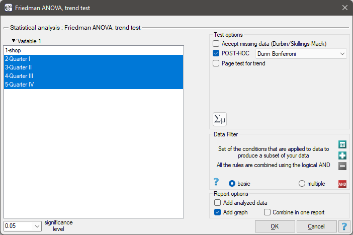
It is possible to take missing data into account by using the Accept missing data option, calculating Durbin ANOVA or Skillings-Mack ANOVA;
it is possible to test the trend in the arrangement of the studied groups by performing Page test for trend.

Basic assumptions:

measurement on an ordinal scale or on an interval scale,
a dependent model.

Hypotheses relate to the equality of the sum of ranks for successive measurements ( $R_{j}$ ) or are simplified to medians ( $\theta_j$ )

$\begin{array}{cl} \mathcal{H}_0: & \theta_1=\theta_2=...=\theta_k,\\ \mathcal{H}_1: & $not all $\theta_j$ are equal $(j=1,2,...,k)$,$ \end{array}$

where:

$\theta_1,\theta_2,...\theta_k$ medians for an analysed features, in the following measurements from the examined population.

Two test statistics are determined: the Friedman statistic and the Iman-Davenport modification of this statistic.

The Friedman statistic has the form:

$\begin{displaymath} T_1=\frac{1}{C}\left(\frac{12}{nk(k+1)}\left(\sum_{j=1}^k\left(\sum_{i=1}^n R_{ij}\right)^2\right)-3n(k+1)\right), \end{displaymath}$

where:

$n$ – sample size,

$R_{ij}$ – ranks ascribed to the following measurements $(j=1,2,...k)$ , separately for the analysed objects $(i=1,2,...n)$ ,

$\displaystyle C=1-\frac{\sum(t^3-t)}{n(k^3-k)}$ – correction for ties,

$t$ – number of cases included in a tie.

The Iman-Davenport modification of the Friedman statistic has the form:

$\begin{displaymath} T_2=\frac{(n_j-1)T_1}{n_j(k-1)-T_1} \end{displaymath}$

The formula for the test statistic $T_1$ and $T_2$ includes the correction for ties $C$ . This correction is used, when ties occur (if there are no ties, the correction is not calculated, because of $C=1$ ).

The $T_1$ statistic has asymptotically (for large sample sizes) has the Chi-square distribution with $df=k - 1$ degrees of freedom.

The statistic $T_2$ follows the Snedecor's F distribution with $df_1=k-1$ i $df_2=(n_j-1)(k-1)$ degrees of freedem.

The p-value, designated on the basis of the test statistic, is compared with the significance level $\alpha$ :

$\begin{array}{ccl} $ if $ p \le \alpha & \Longrightarrow & $ reject $ \mathcal{H}_0 $ and accept $ \mathcal{H}_1, \\ $ if $ p > \alpha & \Longrightarrow & $ there is no reason to reject $ \mathcal{H}_0. \\ \end{array}$

The POST-HOC tests

Introduction to the contrasts and the POST-HOC tests was performed in the unit, which relates to the one-way analysis of variance.

The Dunn test

For simple comparisons (frequency in particular measurements is always the same).

The Dunn test (Dunn 1964³⁾) is a corrected test due to multiple testing. The Bonferroni or Sidak correction is most commonly used here, although other, newer corrections are also available and are described in more detail in the Multiple Comparisons section.

Hypotheses:

Example - simple comparisons (comparison of 2 selected medians):

$\begin{array}{cc} \mathcal{H}_0: & \theta_j=\theta_{j+1},\\ \mathcal{H}_1: & \theta_j \neq \theta_{j+1}. \end{array}$

[i] The value of critical difference is calculated by using the following formula:

$\begin{displaymath} CD=Z_{\frac{\alpha}{c}}\sqrt{\frac{k(k+1)}{6n}}, \end{displaymath}$

where:

$\displaystyle Z_{\frac{\alpha}{c}}$ - is the critical value (statistic) of the normal distribution for a given significance level $\alpha$ corrected on the number of possible simple comparisons $c$ .

[ii] The test statistic is defined by:

$\begin{displaymath} Z=\frac{\sum_{j=1}^k c_jR_j}{\sqrt{\frac{k(k+1)}{6n}}}, \end{displaymath}$

where:

$\overline{R}_j$ – mean of the ranks of the $j$ -th measurement, for $(j=1,2,...k)$ ,

The test statistic asymptotically (for large sample size) has normal distribution, and the p-value is corrected on the number of possible simple comparisons $c$ .

Conover-Inman test

Non-parametric equivalent of Fisher LSD⁴⁾, sed for simple comparisons (counts across measurements are always the same).

[i] he value of critical difference is calculated by using the following formula:

$\begin{displaymath} CD=\sqrt{F_{\alpha,1,df_2}}\cdot\sqrt{\frac{2\left(n_jA-\sum_{j=1}^tR_j^k\right)}{(n_j-1)(k-1)}}, \end{displaymath}$

where:

$\displaystyle A=\sum_{i=1}^{n_j}\sum_{j=1}^kR_{ij}^2$ – sum of squares for ranks,

$\displaystyle F_{\alpha,1,df_2}$ to critical value (statistic) Snedecor's F distribution for a given significance level $\alpha$ and for degrees of freedom respectively: 1 and $df_2$ .

[ii] The test statistic is defined by:

$\begin{displaymath} t=\frac{\sum_{j=1}^k c_jR_j}{\sqrt{\frac{2\left(n_jA-\sum_{j=1}^tR_j^k\right)}{(n_j-1)(k-1)}}}, \end{displaymath}$

where:

$R_j$ – the sum of ranks of $j$ th measurement, for $(j=1,2,...k)$ ,

The test statistic hast-Student distribution with $df_2$ degrees of freedem.

The settings window with the Friedman ANOVA can be opened in Statistics menu→NonParametric tests →Friedman ANOVA, trend test or in ''Wizard''

EXAMPLE (chocolate bar.pqs file)

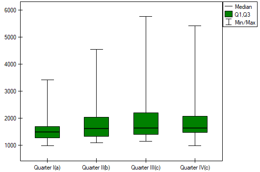
Quarterly sale of some chocolate bar was measured in 14 randomly chosen supermarkets. The study was started in January and finished in December. During the second quarter, the billboard campaign was in full swing. Let's check if the campaign had an influence on the advertised chocolate bar sale.

$\begin{tabular}{|c|c|c|c|c|} \hline Shop&Quarter I&Quarter II&Quarter III&Quarter IV\\\hline SK1&3415&4556&5772&5432\\ SK2&1593&1937&2242&2794\\ SK3&1976&2056&2240&2085\\ SK4&1526&1594&1644&1705\\ SK5&1538&1634&1866&1769\\ SK6&983&1086&1135&1177\\ SK7&1050&1209&1245&977\\ SK8&1861&2087&2054&2018\\ SK9&1714&2415&2361&2424\\ SK10&1320&1621&1624&1551\\ SK11&1276&1377&1522&1412\\ SK12&1263&1279&1350&1490\\ SK13&1271&1417&1583&1513\\ SK14&1436&1310&1357&1468\\\hline \end{tabular}$

Hypotheses:

$\begin{array}{cl} \mathcal{H}_0: & $there is a lack of significant difference in sale values, in the compared $\\ & $quarters, in the population represented by the whole sample, $\\ \mathcal{H}_1: & $the difference in sale values, between at least 2 quarters, is significant,$\\ & $in the population represented by the whole sample.$ \end{array}$

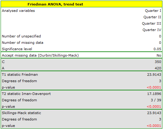
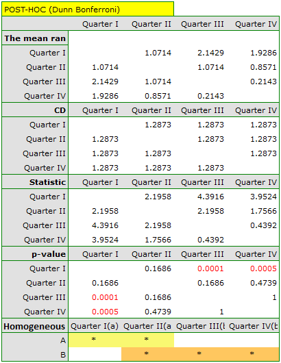
Comparing the p-value of the Friedman test (as well as the p-value of the Iman-Davenport correction of the Friedman test) with a significance level $\alpha=0.05$ , we find that sales of the bar are not the same in each quarter. The POST-HOC Dunn analysis performed with the Bonferroni correction indicates differences in sales volumes pertaining to quarters I and III and I and IV, and an analogous analysis performed with the stronger Conover-Iman test indicates differences between all quarters except quarters III and IV.

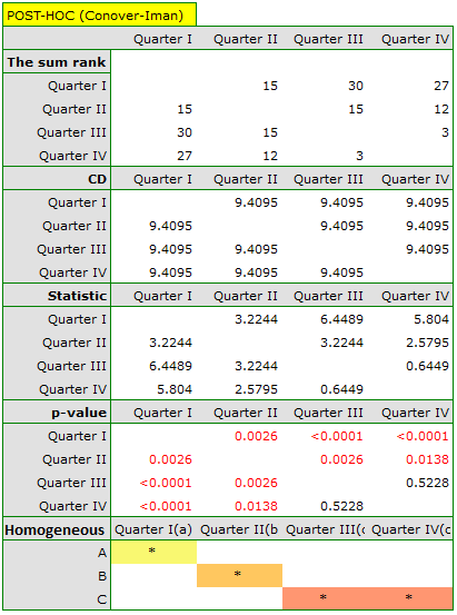
In the graph, we presented homogeneous groups determined by the Conover-Iman test.

We can provide a detailed description of the data by selecting Descriptive statistics in the analysis window .

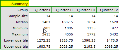
If the data were described by an ordinal scale with few categories, it would be useful to present it also in numbers and percentages. In our example, this would not be a good method of description.

¹⁾

Friedman M. (1937), The use of ranks to avoid the assumption of normality implicit in the analysis of variance. Journal of the American Statistical Association, 32,675-701

²⁾

Iman R. L., Davenport J. M. (1980), Approximations of the critical region of the friedman statistic, Communications in Statistics 9, 571–595

³⁾

Dunn O. J. (1964), Multiple comparisons using rank sums. Technometrics, 6: 241–252

⁴⁾

Conover W. J. (1999), Practical nonparametric statistics (3rd ed). John Wiley and Sons, New York

PQStat - Baza Wiedzy

Narzędzia użytkownika

Narzędzia witryny

Pasek boczny

The Friedman ANOVA

Narzędzia strony