Narzędzia użytkownika
Narzędzia witryny
Pasek boczny
en:statpqpl:zgodnpl
Spis treści
Agreement analysis
{\ovalnode{A}{\hyperlink{rozklad_normalny}{\begin{tabular}{c}Are\\the data\\normally\\distributed?\end{tabular}}}}
\rput[br](3.2,6.2){\rnode{B}{\psframebox{\hyperlink{ICC}{\begin{tabular}{c}test of\\significance\\for the Intraclass\\Correlation\\Coefficient ($r_{ICC}$)\end{tabular}}}}}
\ncline[angleA=-90, angleB=90, arm=.5, linearc=.2]{->}{A}{B}
\rput(2.2,10.4){T}
\rput(4.3,12.5){N}
\rput(7.5,14){\hyperlink{porzadkowa}{Ordinal scale}}
\rput[br](9.4,11.25){\rnode{C}{\psframebox{\hyperlink{Kendall_W}{\begin{tabular}{c}test of\\significance\\for the Kendall's $\widetilde{W}$\\coefficient\end{tabular}}}}}
\ncline[angleA=-90, angleB=90, arm=.5, linearc=.2]{->}{A}{C}
\rput(12.5,14){\hyperlink{nominalna}{Nominal scale}}
\rput[br](14.2,11.25){\rnode{D}{\psframebox{\hyperlink{wspolczynnik_Kappa}{\begin{tabular}{c}test of\\significance\\for the Cohen's $\hat \kappa$\\coefficient\end{tabular}}}}}
\rput(4.8,9.8){\hyperlink{testy_normalnosci}{normality tests}}
\psline[linestyle=dotted]{<-}(3.4,11.2)(4,10)
\end{pspicture}](/lib/exe/fetch.php?media=wiki:latex:/img3a356f241f0fd2e39b213fc95163dc83.png "LaTeX")
Parametric tests
The Intraclass Correlation Coefficient and a test to examine its significance
The intraclass correlation coefficient is used when the measurement of variables is done by a few „raters” ( ). It measures the strength of interrater reliability
  the degree of its assessment concordance.
Since it can be determined in several different situations, there are several variations depending on the model and the type of concordance. Depending on the variability present in the data, we can distinguish between 2 main research models and 2 types of concordance.
Model 1
For each of the  randomly selected judged objects, a set of
  judges is randomly selected from the population of judges. Whereby for each object a different set of judges can be drawn.
The ICC coefficient is then determined by the random model ANOVA for independent groups. The question of the reliability of a single judge's ratings is answered by ICC(1,1) given by the formula:

To estimate the reliability of scores that are the average of the judges' ratings (for judges), determine ICC(1,k) given by the formula:

where:
 – mean of squares within groups,
 – mean of squares between objects.
Model 2
A set of judges is randomly selected from a population of judges and each judge evaluates all random objects.
The ICC coefficient is then determined in a random model ANOVA for dependent groups.
Depending on the type of concordance we are looking for, we can estimate: absolute agreement, i.e., if the judges agree absolutely, they give exactly the same ratings, e.g., perfectly concordant will be such ratings given by a pair of judges (2,2), (5,5), (8,8); or consistency, i.e., the judges may use different ranges of values but beyond this shift there should be no differences to keep the verdict consistent, e.g., perfectly consistent will be such ratings given by a pair of judges (2,5), (5,8), (8,11).
- Absolute agreement
The question about the reliability of a single judge's ratings is answered by ICC(2,1) given by the formula:

To estimate the reliability of scores that are the average of the judges' ratings (for judges), determine ICC(2,k) given by the formula:

where:
 – the mean of squares between judges,
 – the mean of squares between objects,
 – mean of squares for the residuals.
- Consistency
The question about the reliability of a single judge's ratings is answered by ICC(2,1) given by the formula:

To estimate the reliability of scores that are the average of the judges' ratings (for judges), determine ICC(2,k) given by the formula:

where:
– the mean of squares between objects,
– mean of squares for the residuals.
Note
Sometimes, there is a need to consider model 3 1), i.e., a set of judges is selected and each judge evaluates all random objects. The concordance score applies only to these particular judges. The ICC coefficient is then determined in a mixed model (since the randomness only affects the objects and not the judges). Since we are ignoring the variability concerning the judges, we are examining consistency (rather than absolute agreement) and the coefficients from the second model may apply: ICC(2,1) and ICC (2,k), since they are the same as the coefficients ICC(3,1) and ICC (3,k) desired in this case under the assumption of no interaction between objects and judges.
Note
We interpret the value  as follows:
 it is an strong concordance of objects assessment made by judgess; it is especially reflected in a high-variance between objects (a significant means difference between objects) and a low-variance between judges assessments (a small means difference of assessments designated by judges);
 a negative intraclass coefficient is treated in the same ways as
  ;
; denotes a lack of concordance in the judges' evaluations of individual objects, as reflected by low variance between objects (a small difference in means between objects) and high variance between judges' evaluations (a significant difference in mean scores determined for judges).
F-test for testing the significance of intraclass correlation coefficient
Basic assumptions:
- measurement on an interval scale,
- the normal distribution for all variables which are the differences of measurement pairs (or the normal distribution for an analysed variable in each measurement),
- for model 1 - independent model, for model 2 / 3 - dependent model.
Hypotheses:

The test statistic has the form:

or

This statistic has the F Snedecor distribution with the number of degrees of freedom defined in the model.
The p-value, designated on the basis of the test statistic, is compared with the significance level  :
:

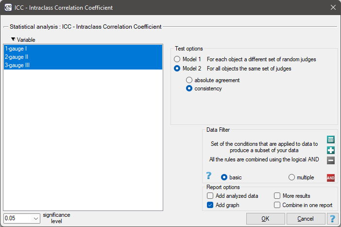
The settings window with the ICC – Intraclass Correlation Coefficient can be opened in Statistics menu→Parametric tests→ICC – Intraclass Correlation Coefficient or in ''Wizard''.
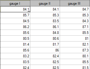
EXAMPLE (sound intensity.pqs file)
In order to effectively care for the hearing of workers in the workplace, it is first necessary to reliably estimate the sound intensity in the various areas where people are present. One company decided to conduct an experiment before choosing a sound intensity meter (sonograph). Measurements of sound intensity were made at 42 randomly selected measurement points in the plant using 3 drawn analog sonographs and 3 randomly selected digital sonographs. A part of collected measurements is presented in the table below.
To find out which type of instrument (analog or digital) will better accomplish the task at hand, the ICC in model 2 should be determined by examining the absolute agreement. The type of meter with the higher ICC will have more reliable measurements and will therefore be used in the future.
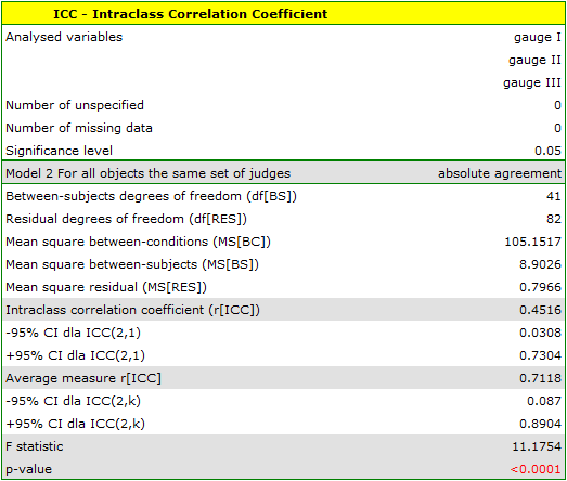
The analysis performed for the analog meters shows significant consistency of the measurements (p<0.0001). The reliability of the measurement made by the analog meter is ICC(2,1) = 0.45, while the reliability of the measurement that is the average of the measurements made by the 3 analog meters is slightly higher and is ICC(2,k) = 0.71. However, the lower limit of the 95 percent confidence interval for these coefficients is disturbingly low.
A similar analysis performed for digital meters produced better results. The model is again statistically significant, but the ICC coefficients and their confidence intervals are much higher than for analog meters, so the absolute agreement obtained is higher ICC(2,1) = 0.73, ICC(2,k) = 0.89.
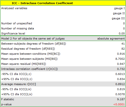
Therefore, eventually digital meters will be used in the workplace.
The agreement of the results obtained for the digital meters is shown in a dot plot, where each measurement point is described by the sound intensity value obtained for each meter.
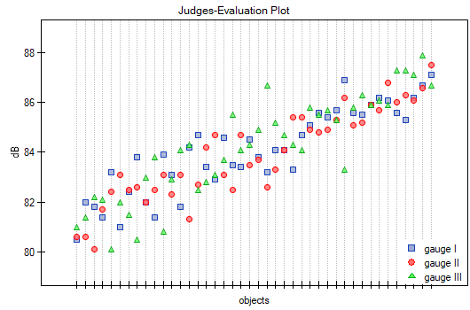
By presenting a graph for the previously sorted data according to the average value of the sound intensity, one can check whether the degree of agreement increases or decreases as the sound intensity increases. In the case of our data, a slightly higher correspondence (closeness of positions of points on the graph) is observed at high sound intensities.
Similarly, the consistency of the results obtained can be observed in the Blanda-Altmana graphs2) constructed separately for each pair of meters. The graph for Meter I and Meter II is shown below.
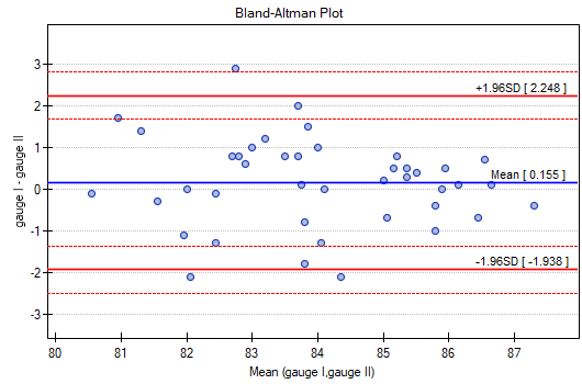
Here, too, we observe higher agreement (points are concentrated near the horizontal axis y=0) for higher sound intensity values.
Note
If the researcher was not concerned with estimating the actual sound level at the worksite, but wanted to identify where the sound level was higher than at other sites or to see if the sound level varied over time, then Model 2, which tests consistency, would be a sufficient model.
Non-parametric tests
The Kendall's concordance coefficient and a test to examine its significance
The Kendall's  coefficient of concordance is described in the works of Kendall, Babington-Smith (1939)3) and Wallis (1939)4). It is used when the result comes from different sources (from different raters) and concerns a few () objects. However, the assessment concordance is necessary. Is often used in measuring the interrater reliability strength – the degree of (raters) assessment concordance.
The Kendall's coefficient of concordance is calculated on an ordinal scale or a interval scale. Its value is calculated according to the following formula:

where:
– number of different assessments sets (the number of raters),
– number of ranked objects,
 ,
,
 – ranks ascribed to the following objects
  , independently for each rater
  ,
,
 – a correction for ties,
 – number of cases incorporated into tie.
The coefficient's formula includes  – the correction for ties. This correction is used, when ties occur (if there are no ties, the correction is not calculated, because of
  ).
).
Note
 – the Kendall's coefficient in a population;
– the Kendall's coefficient in a sample.
The value of  and it should be interpreted in the following way:
 means a strong concordance in raters assessments;
 means a lack of concordance in raters assessments.
The Kendall's W coefficient of concordance vs. the Spearman coefficient:
- When the values of the Spearman
 correlation coefficient (for all possible pairs) are calculated, the average coefficient – marked by
  is a linear function of coefficient:

The Kendall's W coefficient of concordance vs. the Friedman ANOVA:
- The Kendall's coefficient of concordance and the Friedman ANOVA are based on the same mathematical model. As a result, the value of the chi-square test statistic for the Kendall's coefficient of concordance and the value of the chi-square test statistic for the Friedman ANOVA are the same.
The chi-square test of significance for the Kendall's coefficient of concordance
Basic assumptions:
- measurement on an ordinal scale or on an interval scale.
Hypotheses:

The test statistic is defined by:
 This statistic asymptotically (for large sample sizes) has the Chi-square distribution with the degrees of freedom calculated according to the following formula:
  .
.
The p-value, designated on the basis of the test statistic, is compared with the significance level :
The settings window with the test of the Kendall's W significance can be opened in Statistics menu →NonParametric tests→Kendall's W or in ''Wizard''.
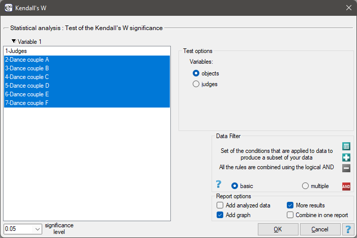
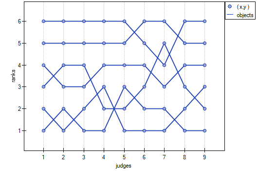
In the 6.0 system, dancing pairs grades are assessed by 9 judges. The judges point for example an artistic expression. They asses dancing pairs without comparing each of them and without placing them in the particular „podium place” (they create a ranking). Let's check if the judges assessments are concordant.

Hypotheses:

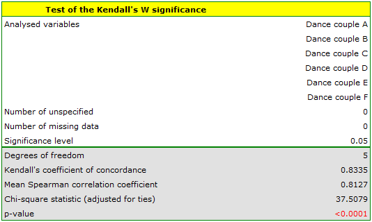
Comparing the p <0.0001 with the significance level  , we have stated that the judges assessments are statistically concordant. The concordance strength is high:
  , similarly the average Spearman's rank-order correlation coefficient:
  . This result can be presented in the graph, where the X-axis represents the successive judges. Then the more intersection of the lines we can see (the lines should be parallel to the X axis, if the concordance is perfect), the less there is the concordance of rateres evaluations.
The Cohen's Kappa coefficient and the test examining its significance
The Cohen's Kappa coefficient (Cohen J. (1960)5)) defines the agreement level of two-times measurements of the same variable in different conditions. Measurement of the same variable can be performed by 2 different observers (reproducibility) or by a one observer twice (recurrence). The  coefficient is calculated for categorial dependent variables and its value is included in a range from -1 to 1. A 1 value means a full agreement, 0 value means agreement on the same level which would occur for data spread in a contingency table randomly. The level between 0 and -1 is practically not used. The negative value means an agreement on the level which is lower than agreement which occurred for the randomly spread data in a contingency table. The coefficient can be calculated on the basis of raw data or a
  contingency table.
Unweighted Kappa (i.e., Cohen's Kappa) or weighted Kappa can be determined as needed. The assigned weights ( ) refer to individual cells of the contingency table, on the diagonal they are 1 and off the diagonal they belong to the range
  .
.
Unweighted Kappa
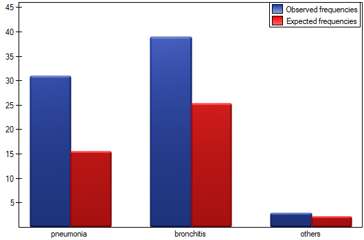
It is calculated for data, the categories of which cannot be ordered, e.g. data comes from patients, who are divided according to the type of disease which was diagnosed, and these diseases cannot be ordered, e.g. pneumonia  , bronchitis
  and other
  . In such a situation, one can check the concordance of the diagnoses given by the two doctors by using unweighted Kappa, or Cohen's Kappa. Discordance of pairs
  and
and  will be treated equivalently, so the weights off the diagonal of the weight matrix will be zeroed.
Weighted Kappa
In situations where data categories can be sorted, e.g., data comes from patients who are divided by the lesion grade into: no lesion , benign lesion , suspected cancer , cancer  , one can build the concordance of the ratings given by the two radiologists taking into account the possibility of sorting. The ratings of
  than may then be considered as more discordant pairs of ratings. For this to be the case, so that the order of the categories affects the compatibility score, the weighted Kappa should be determined.
The assigned weights can be in linear or quadratic form.
- Linear weights (Cicchetti, 19716)) – calculated according to the formula:

The greater the distance from the diagonal of the matrix the smaller the weight, with the weights decreasing proportionally. Example weights for matrices of size 5×5 are shown in the table:

- Square weights (Cohen, 19687)) – calculated according to the formula:

The greater the distance from the diagonal of the matrix, the smaller the weight, with weights decreasing more slowly at closer distances from the diagonal and more rapidly at farther distances. Example weights for matrices of size 5×5 are shown in the table:

Quadratic scales are of greater interest because of the practical interpretation of the Kappa coefficient, which in this case is the same as the intraclass correlation coefficient 8).
To determine the Kappa coefficient compliance, the data are presented in the form of a table of observed counts  , and this table is transformed into a probability contingency table
  .
.
The Kappa coefficient () is expressed by the formula:

where:
 ,
,
 ,
,
 ,
,  - total sums of columns and rows of the probability contingency table.
Note
denotes the concordance coefficient in the sample, while  in the population.
The standard error for Kappa is expressed by the formula:
![\begin{displaymath}
SE_{\hat \kappa}=\frac{1}{(1-P_e)\sqrt{n}}\sqrt{\sum_{i=1}^{c}\sum_{j=1}^{c}p_{i.}p_{.j}[w_{ij}-(\overline{w}_{i.}+(\overline{w}_{.j})]^2-P_e^2}
\end{displaymath}](/lib/exe/fetch.php?media=wiki:latex:/img059555813b7a0927359f9000c829f6fe.png "LaTeX")
where:
 ,
,
 .
.
The Z test of significance for the Cohen's Kappa () (Fleiss,20039)) is used to verify the hypothesis informing us about the agreement of the results of two-times measurements  and
and  features
  and it is based on the coefficient calculated for the sample.
Basic assumptions:
- measurement on a nominal scale (unweighted Kappa) or on a ordinal scale (unweighted Kappa).
Hypotheses:

The test statistic is defined by:

Where:
![$\displaystyle{SE_{\kappa_{distr}}=\frac{1}{(1-P_e)\sqrt{n}}\sqrt{\sum_{i=1}^c\sum_{j=1}^c p_{ij}[w_{ij}-(\overline{w}_{i.}+\overline{w}_{.j})(1-\hat \kappa)]^2-[\hat \kappa-P_e(1-\hat \kappa)]^2}}$](/lib/exe/fetch.php?media=wiki:latex:/imgc30723ad5a68d25b44687da3bff2c069.png "LaTeX") .
.
The  statistic asymptotically (for a large sample size) has the normal distribution.
The p-value, designated on the basis of the test statistic, is compared with the significance level :
The settings window with the test of Cohen's Kappa significance can be opened in Statistics menu → NonParametric tests → Kappa-Cohen or in ''Wizard''.
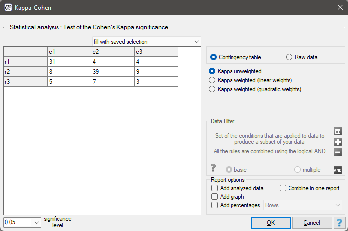
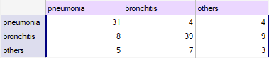
You want to analyse the compatibility of a diagnosis made by 2 doctors. To do this, you need to draw 110 patients (children) from a population. The doctors treat patients in a neighbouring doctors' offices. Each patient is examined first by the doctor A and then by the doctor B. Both diagnoses, made by the doctors, are shown in the table below.
Hypotheses:
We could analyse the agreement of the diagnoses using just the percentage of the compatible values. In this example, the compatible diagnoses were made for 73 patients (31+39+3=73) which is 66.36% of the analysed group. The kappa coefficient introduces the correction of a chance agreement (it takes into account the agreement occurring by chance).
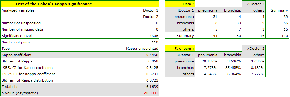
The agreement with a chance adjustment  is smaller than the one which is not adjusted for the chances of an agreement.
The p<0.0001. Such result proves an agreement between these 2 doctors' opinions, on the significance level ,.
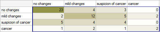
Radiological imaging assessed liver damage in the following categories: no changes (1), mild changes (2), suspicion of cancer , cancer . The evaluation was done by two independent radiologists based on a group of 70 patients. We want to check the concordance of the diagnosis.
Hypotheses:
Because the diagnosis is issued on an ordinal scale, an appropriate measure of concordance would be the weighted Kappa coefficient.
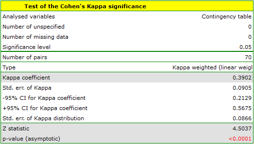
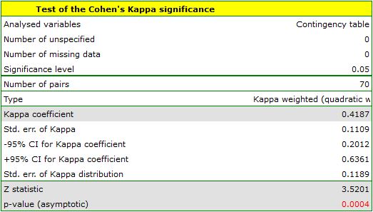
Because the data are mainly concentrated on the main diagonal of the matrix and in close proximity to it, the coefficient weighted by the linear weights is lower ( ) than the coefficient determined for the quadratic weights (
 ). In both situations, this is a statistically significant result (at the significance level), p<0.0001.
If there was a large disagreement in the ratings concerning the two extreme cases and the pair: (no change and cancer) located in the upper right corner of the table occurred far more often, e.g., 15 times, then such a large disagreement would be more apparent when using quadratic weights (the Kappa coefficient would drop dramatically) than when using linear weights.
The Kappa Fleiss coefficient and a test to examine its significance
This coefficient determines the concordance of measurements conducted by a few judges (Fleiss, 197110)) and is an extension of Cohen's Kappa coefficient, which allows testing the concordance of only two judges. With that said, it should be noted that each of randomly selected objects can be judged by a different random set of judges. The analysis is based on data transformed into a table with rows and  columns, where is the number of possible categories to which the judges assign the test objects. Thus, each row in the table gives
  , which is the number of judges making the judgments specified in that column.
The Kappa coefficient () is then expressed by the formula:
where:
 ,
,
 ,
,
 .
.
A value of  indicates full agreement among judges, while
  indicates the concordance that would arise if the judges' opinions were given at random. Negative values of Kappa, on the other hand, indicate concordance less than that at random.
For a coefficient of the standard error  can be determined, which allows statistical significance to be tested and asymptotic confidence intervals to be determined.
Z test for significance of Fleiss' Kappa coefficient () (Fleiss, 200311)) is used to test the hypothesis that the ratings of several judges are consistent and is based on the coefficient calculated for the sample.
Basic assumptions:
- measurement on a nominal scale – possible category ordering is not taken into account.
Hypotheses:
The test statistic has the form:

The statistic asymptotically (for large sample sizes) has the normal distribution.
The p-value, designated on the basis of the test statistic, is compared with the significance level :
Note
The determination of Fleiss's Kappa coefficient is conceptually similar to the Mantel-Haenszel method. The determined Kappa is a general measure that summarizes the concordance of all judge ratings and can be determined as the Kappa formed from individual layers, which are specific judge ratings (Fleiss, 200312)). Therefore, as a summary of each layer, the judges' concordance (Kappa coefficient) can be determined summarizing each possible rating separately.
The settings window with the test of the Fleiss's Kappa significance can be opened in Statistics menu →NonParametric tests→Fleiss Kappa.
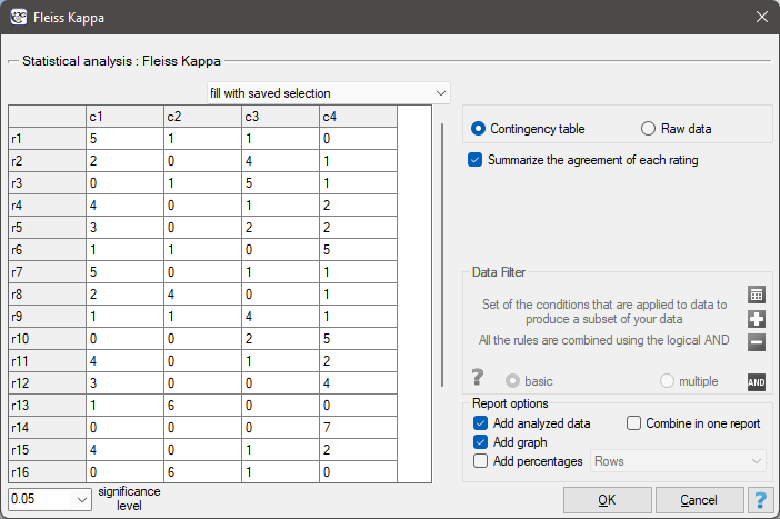
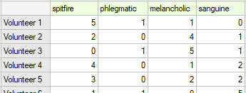
EXAMPLE (temperament.pqs file)
20 volunteers take part in a game to determine their personality type. Each volunteer has a rating given by 7 different observers (usually people from their close circle or family). Each observer has been introduced to the basic traits describing temperament in each personality type: choleric, phlegmatic, melancholic, sanguine. We examine observers' concordance in assigning personality types. An excerpt of the data is shown in the table below.}
Hypotheses:
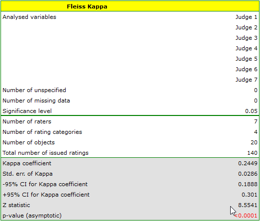
We observe an unimpressive Kappa coefficient = 0.24, but statistically significant (p<0.0001), indicating non-random agreement between judges' ratings. The significant concordance applies to each grade, as evidenced by the concordance summary report for each stratum (for each grade) and the graph showing the individual Kappa coefficients and Kappa summarizing the total.
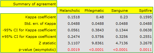
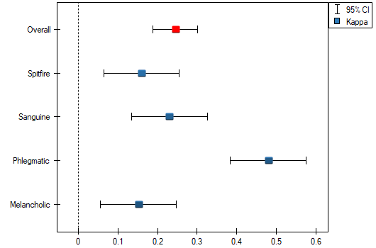
It may be interesting to note that the highest concordance is for the evaluation of phlegmatics (Kappa=0.48).
With a small number of people observed, it is also useful to make a graph showing how observers rated each person.
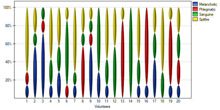
In this case, only person no 14 received an unambiguous personality type rating – sanguine. Person no. 13 and 16 were assessed as phlegmatic by 6 observers (out of 7 possible). In the case of the remaining persons, there was slightly less agreement in the ratings. The most difficult to define personality type seems to be characteristic of the last person, who received the most diverse set of ratings.
1)
Shrout P.E., and Fleiss J.L (1979), Intraclass correlations: uses in assessing rater reliability. Psychological Bulletin, 86, 420-428
2)
Bland J.M., Altman D.G. (1999), Measuring agreement in method comparison studies. Statistical Methods in Medical Research 8:135-160.
3)
Kendall M.G., Babington-Smith B. (1939), The problem of m rankings. Annals of Mathematical Statistics, 10, 275-287
4)
Wallis W.A. (1939), The correlation ratio for ranked data. Journal of the American Statistical Association, 34,533-538
5)
Cohen J. (1960), A coefficient of agreement for nominal scales. Educational and Psychological Measurement, 10,3746
6)
Cicchetti D. and Allison T. (1971), A new procedure for assessing reliability of scoring eeg sleep recordings. American Journal EEG Technology, 11, 101-109
7)
Cohen J. (1968), Weighted kappa: nominal scale agreement with provision for scaled disagreement or partial credit. Psychological Bulletin, 70, 213-220
8)
Fleiss J.L., Cohen J. (1973), The equivalence of weighted kappa and the intraclass correlation coeffcient as measure of reliability. Educational and Psychological Measurement, 33, 613-619
9)
, 11)
, 12)
Fleiss J.L., Levin B., Paik M.C. (2003), Statistical methods for rates and proportions. 3rd ed. (New York: John Wiley) 598-626
10)
Fleiss J.L. (1971), Measuring nominal scale agreement among many raters. Psychological Bulletin, 76 (5): 378–382
en/statpqpl/zgodnpl.txt · ostatnio zmienione: 2022/02/13 20:56 przez admin
Narzędzia strony
Wszystkie treści w tym wiki, którym nie przyporządkowano licencji, podlegają licencji: CC Attribution-Noncommercial-Share Alike 4.0 International
