Narzędzia użytkownika
Narzędzia witryny
Pasek boczny
en:statpqpl:rozkladypl:kalkupl
Probability distribution calculator
The area under a curve (density function) is  probability of occurrence of all possible values of an analysed random variable. The whole area under a curve comes to
  . If you want to analyse just a part of this area, you must put the border value, which is called the critical value or
 Statistic. To do this, you need to open the Probability distribution calculator window. In this window you can calculate not only a value of the area under the curve (p-value) of the given distribution on the basis of Statistic, but also Statistic value on the basis of p-value. To open the window of Probability distribution calculator, you need to select Probability distribution calculator from the Statistics→Calculators menu.
EXAMPLE Probability distribution calculator
Some mobile network operator did the research, which was supposed to show the usage of „free minutes” given to his clients on a pay-monthly contract. On the basis of the sample, which consists of 200 of the above-mentioned network clients (where the distribution of used free minutes is of the shape of normal distribution) is calculated the mean value  and standard deviation
  We want to calculate the probability, that the chosen client used:
- 150 minutes or less,
- more than 150 minutes,
- the amount of minutes coming from the range
![$[\overline{x}- sd,\overline{x}+ sd] =[148.12min.,174.18min.]$](/lib/exe/fetch.php?media=wiki:latex:/imge95ee390798d5f324a87a7ff392a75a6.png "LaTeX") ,
, - the amount of minutes out of the range
 .
.
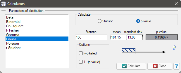
Open the Probability distribution calculator window, select Gaussian distribution and write the mean  and
and standard deviation  and select the option which indicates, that you are going to calculate the
 p- value.
(1)To calculate (using normal distribution (Gauss)) the probability that the client you have chosen used 150 free minutes or less, put the value of 150 in the Statistic field. Confirm all selected settings by clicking Calculate.
![\psset{xunit=1.2cm,yunit=8cm}
\begin{pspicture}(-3.5,-.05)(4.2,0.4)
\psline{-}(-4,0)(4,0)
\psGauss[linecolor=blue, mue=0, sigma=1]{-4}{4}%
\pscustom[fillstyle=solid,fillcolor=red!30]{%
\psGauss[linewidth=1pt,mue=0, sigma=1]{-4}{-0.85572}%
\psline(-0.85572,0)(-4,0)}
\rput(2.4,0.25){\textcolor{blue}{$N(161.15,13.03)$}}
\rput(-0.85572,-0.05){\textcolor{blue}{150}}
\end{pspicture}](/lib/exe/fetch.php?media=wiki:latex:/img3c7c1127f8168931642e12a3d7aae440.png "LaTeX")
The obtained p-value is 0.193961.
Note
Similar calculations you can carry out on the basis of empirical distribution. The only thing you should do is to calculate a percentage of clients who use 150 minutes or less (example (\ref{tab_licznosci}) by using the Frequency tables window. In the analysed sample (which consists of 200 clients) there are 40 clients who use 150 minutes or less. It is 20% of the whole sample, so the probability you are looking for is  .
.
(2) To calculate the probability (using the normal distribution (Gauss)), that the client who you have chosen used more than 150 free minutes, you need to put the value of 150 in the Statistic field and than select the option 1 - (p-value). Confirm all the chosen settings by clicking Calculate.
![\psset{xunit=1.2cm,yunit=8cm}
\begin{pspicture}(-3.5,-.05)(4.2,0.4)
\psline{-}(-4,0)(4,0)
\psGauss[linecolor=blue, mue=0, sigma=1]{-4}{4}%
\pscustom[fillstyle=solid,fillcolor=red!30]{%
\psline(-0.85572,0)(-0.85572,0)%
\psGauss[linewidth=1pt,mue=0, sigma=1]{-0.85572}{4}%
\psline(4,0)(-0.85572,0)}
\rput(2.4,0.25){\textcolor{blue}{$N(161.15,13.03)$}}
\rput(-0.85572,-0.05){\textcolor{blue}{150}}
\end{pspicture}](/lib/exe/fetch.php?media=wiki:latex:/img880f38e5b626288ec2683062b11adc2f.png "LaTeX")
The obtained p-value is 0.806039.
(3) To calculate (using the normal distribution (Gauss)) a probability that the client you have chosen used free minutes which come from the range in the Statistic field, put one of the final range values and than select the option two-sided. Confirm all the chosen settings by clicking Calculate.
![\psset{xunit=1.2cm,yunit=8cm}
\begin{pspicture}(-3.5,-.05)(4.2,0.4)
\psline{-}(-4,0)(4,0)
\psGauss[linecolor=blue, mue=0, sigma=1]{-4}{4}%
\pscustom[fillstyle=solid,fillcolor=red!30]{%
\psline(-1,0)(-1,0)%
\psGauss[linewidth=1pt,mue=0, sigma=1]{-1}{1}%
\psline(1,0)(-1,0)}
\rput(2.4,0.25){\textcolor{blue}{$N(161.15,13.03)$}}
\rput(-1,-0.05){\textcolor{blue}{148.12}}
\rput(1,-0.05){\textcolor{blue}{174.18}}
\end{pspicture}](/lib/exe/fetch.php?media=wiki:latex:/imgc26fc1da363b6ae663ba5efe85065299.png "LaTeX")
The obtained p-value is 0.682689.
(4) To calculate (using the normal distribution (Gauss)) a probability, that the client you have chosen used free minutes out of the range in the Statistic field put one of the final range values and than select the option: two-sided and 1 - (p-value). Confirm all the chosen settings by clicking Calculate.
![\psset{xunit=1.2cm,yunit=8cm}
\begin{pspicture}(-3.5,-.05)(4.2,0.4)
\psline{-}(-4,0)(4,0)
\psGauss[linecolor=blue, mue=0, sigma=1]{-4}{4}%
\pscustom[fillstyle=solid,fillcolor=red!30]{%
\psGauss[linewidth=1pt,mue=0, sigma=1]{-4}{-1}%
\psline(-1,0)(-4,0)}
\pscustom[fillstyle=solid,fillcolor=red!30]{%
\psline(1,0)(1,0)%
\psGauss[linewidth=1pt,mue=0, sigma=1]{1}{4}%
\psline(4,0)(1,0)}
\rput(2.4,0.25){\textcolor{blue}{$N(161.15,13.03)$}}\rput(-1,-0.05){\textcolor{blue}{148.12}}
\rput(1,-0.05){\textcolor{blue}{174.18}}
\end{pspicture}](/lib/exe/fetch.php?media=wiki:latex:/img65581d342db71d064052a88b203192c0.png "LaTeX")
The obtained p-value is 0.317311.
en/statpqpl/rozkladypl/kalkupl.txt · ostatnio zmienione: 2022/02/11 12:33 przez admin
Narzędzia strony
Wszystkie treści w tym wiki, którym nie przyporządkowano licencji, podlegają licencji: CC Attribution-Noncommercial-Share Alike 4.0 International
