Spis treści

Spatial autocorrelation
- Global Moran's I statistic
- Global Geary's C statistic

Spatial autocorrelation

To conduct spatial autocorrelation on the basis of a Map data we should have at our disposal a point, multipoint, or polygonal file. In the case of an analysis of a polygonal file based on the calculation of objects distances, calculations are based on centroids of polygons, and in the case of a multipoint file they are based on centers of objects.

An analysis of the phenomenon of autocorrelation is based on values assigned to spatial objects. Spatial autocorrelation means that the values of geographically near objects are more similar to one another than those of remote objects. The phenomenon causes the creation of spatial clusters with similar values.

Spatial autocorrelation may not occur – we then speak of spatial randomness. The obtained spatial distribution is as probable as any other distribution. When the neighboring values are similar to one another we can speak about positive autocorrelation. Negative autocorrelation occurs when the values of neighboring areas are more varied than in the case of random distribution.

$\begin{tabular}{|c|c|c|c|c|c|c|c|} \hline \multicolumn{1}{>{\columncolor[rgb]{0.8,0.8,0.8}}l|}{\textcolor[rgb]{0.8,0.8,0.8}i}&\textcolor[rgb]{1,1,1}i&\multicolumn{1}{>{\columncolor[rgb]{0.8,0.8,0.8}}l|}{\textcolor[rgb]{0.8,0.8,0.8}i}&\textcolor[rgb]{1,1,1}i&\multicolumn{1}{>{\columncolor[rgb]{0.8,0.8,0.8}}l|}{\textcolor[rgb]{0.8,0.8,0.8}i}&\textcolor[rgb]{1,1,1}i&\multicolumn{1}{>{\columncolor[rgb]{0.8,0.8,0.8}}l|}{\textcolor[rgb]{0.8,0.8,0.8}i}&\textcolor[rgb]{1,1,1}i\\ \hline \textcolor[rgb]{1,1,1}i&\multicolumn{1}{>{\columncolor[rgb]{0.8,0.8,0.8}}l|}{\textcolor[rgb]{0.8,0.8,0.8}i}&\textcolor[rgb]{1,1,1}i&\multicolumn{1}{>{\columncolor[rgb]{0.8,0.8,0.8}}l|}{\textcolor[rgb]{0.8,0.8,0.8}i}&\textcolor[rgb]{1,1,1}i&\multicolumn{1}{>{\columncolor[rgb]{0.8,0.8,0.8}}l|}{\textcolor[rgb]{0.8,0.8,0.8}i}&\textcolor[rgb]{1,1,1}i&\multicolumn{1}{>{\columncolor[rgb]{0.8,0.8,0.8}}l|}{\textcolor[rgb]{0.8,0.8,0.8}i}\\ \hline \multicolumn{1}{| >{\columncolor[rgb]{0.8,0.8,0.8}}l|}{\textcolor[rgb]{0.8,0.8,0.8}i}&\textcolor[rgb]{1,1,1}i&\multicolumn{1}{>{\columncolor[rgb]{0.8,0.8,0.8}}l|}{\textcolor[rgb]{0.8,0.8,0.8}i}&\textcolor[rgb]{1,1,1}i&\multicolumn{1}{>{\columncolor[rgb]{0.8,0.8,0.8}}l|}{\textcolor[rgb]{0.8,0.8,0.8}i}&\textcolor[rgb]{1,1,1}i&\multicolumn{1}{>{\columncolor[rgb]{0.8,0.8,0.8}}l|}{\textcolor[rgb]{0.8,0.8,0.8}i}&\textcolor[rgb]{1,1,1}i\\ \hline \textcolor[rgb]{1,1,1}i&\multicolumn{1}{>{\columncolor[rgb]{0.8,0.8,0.8}}l|}{\textcolor[rgb]{0.8,0.8,0.8}i}&\textcolor[rgb]{1,1,1}i&\multicolumn{1}{>{\columncolor[rgb]{0.8,0.8,0.8}}l|}{\textcolor[rgb]{0.8,0.8,0.8}i}&\textcolor[rgb]{1,1,1}i&\multicolumn{1}{>{\columncolor[rgb]{0.8,0.8,0.8}}l|}{\textcolor[rgb]{0.8,0.8,0.8}i}&\textcolor[rgb]{1,1,1}i&\multicolumn{1}{>{\columncolor[rgb]{0.8,0.8,0.8}}l|}{\textcolor[rgb]{0.8,0.8,0.8}i}\\ \hline \multicolumn{1}{| >{\columncolor[rgb]{0.8,0.8,0.8}}l|}{\textcolor[rgb]{0.8,0.8,0.8}i}&\textcolor[rgb]{1,1,1}i&\multicolumn{1}{>{\columncolor[rgb]{0.8,0.8,0.8}}l|}{\textcolor[rgb]{0.8,0.8,0.8}i}&\textcolor[rgb]{1,1,1}i&\multicolumn{1}{>{\columncolor[rgb]{0.8,0.8,0.8}}l|}{\textcolor[rgb]{0.8,0.8,0.8}i}&\textcolor[rgb]{1,1,1}i&\multicolumn{1}{>{\columncolor[rgb]{0.8,0.8,0.8}}l|}{\textcolor[rgb]{0.8,0.8,0.8}i}&\textcolor[rgb]{1,1,1}i\\ \hline \textcolor[rgb]{1,1,1}i&\multicolumn{1}{>{\columncolor[rgb]{0.8,0.8,0.8}}l|}{\textcolor[rgb]{0.8,0.8,0.8}i}&\textcolor[rgb]{1,1,1}i&\multicolumn{1}{>{\columncolor[rgb]{0.8,0.8,0.8}}l|}{\textcolor[rgb]{0.8,0.8,0.8}i}&\textcolor[rgb]{1,1,1}i&\multicolumn{1}{>{\columncolor[rgb]{0.8,0.8,0.8}}l|}{\textcolor[rgb]{0.8,0.8,0.8}i}&\textcolor[rgb]{1,1,1}i&\multicolumn{1}{>{\columncolor[rgb]{0.8,0.8,0.8}}l|}{\textcolor[rgb]{0.8,0.8,0.8}i}\\ \hline \multicolumn{1}{| >{\columncolor[rgb]{0.8,0.8,0.8}}l|}{\textcolor[rgb]{0.8,0.8,0.8}i}&\textcolor[rgb]{1,1,1}i&\multicolumn{1}{>{\columncolor[rgb]{0.8,0.8,0.8}}l|}{\textcolor[rgb]{0.8,0.8,0.8}i}&\textcolor[rgb]{1,1,1}i&\multicolumn{1}{>{\columncolor[rgb]{0.8,0.8,0.8}}l|}{\textcolor[rgb]{0.8,0.8,0.8}i}&\textcolor[rgb]{1,1,1}i&\multicolumn{1}{>{\columncolor[rgb]{0.8,0.8,0.8}}l|}{\textcolor[rgb]{0.8,0.8,0.8}i}&\textcolor[rgb]{1,1,1}i\\ \hline \textcolor[rgb]{1,1,1}i&\multicolumn{1}{>{\columncolor[rgb]{0.8,0.8,0.8}}l|}{\textcolor[rgb]{0.8,0.8,0.8}i}&\textcolor[rgb]{1,1,1}i&\multicolumn{1}{>{\columncolor[rgb]{0.8,0.8,0.8}}l|}{\textcolor[rgb]{0.8,0.8,0.8}i}&\textcolor[rgb]{1,1,1}i&\multicolumn{1}{>{\columncolor[rgb]{0.8,0.8,0.8}}l|}{\textcolor[rgb]{0.8,0.8,0.8}i}&\textcolor[rgb]{1,1,1}i&\multicolumn{1}{>{\columncolor[rgb]{0.8,0.8,0.8}}l|}{\textcolor[rgb]{0.8,0.8,0.8}i}\\ \hline \end{tabular}$ $\begin{tabular}{|c|c|c|c|c|c|c|c|} \hline \multicolumn{1}{| >{\columncolor[rgb]{0.8,0.8,0.8}}l|}{\textcolor[rgb]{0.8,0.8,0.8}i}&\textcolor[rgb]{1,1,1}i&\textcolor[rgb]{1,1,1}i&\multicolumn{1}{>{\columncolor[rgb]{0.8,0.8,0.8}}l|}{\textcolor[rgb]{0.8,0.8,0.8}i}&\textcolor[rgb]{1,1,1}i&\textcolor[rgb]{1,1,1}i&\multicolumn{1}{>{\columncolor[rgb]{0.8,0.8,0.8}}l|}{\textcolor[rgb]{0.8,0.8,0.8}i}&\textcolor[rgb]{1,1,1}i\\ \hline \textcolor[rgb]{1,1,1}i&\multicolumn{1}{>{\columncolor[rgb]{0.8,0.8,0.8}}l|}{\textcolor[rgb]{0.8,0.8,0.8}i}&\multicolumn{1}{>{\columncolor[rgb]{0.8,0.8,0.8}}l|}{\textcolor[rgb]{0.8,0.8,0.8}i}&\textcolor[rgb]{1,1,1}i&\multicolumn{1}{>{\columncolor[rgb]{0.8,0.8,0.8}}l|}{\textcolor[rgb]{0.8,0.8,0.8}i}&\multicolumn{1}{>{\columncolor[rgb]{0.8,0.8,0.8}}l|}{\textcolor[rgb]{0.8,0.8,0.8}i}&\textcolor[rgb]{1,1,1}i&\multicolumn{1}{>{\columncolor[rgb]{0.8,0.8,0.8}}l|}{\textcolor[rgb]{0.8,0.8,0.8}i}\\ \hline \textcolor[rgb]{1,1,1}i&\textcolor[rgb]{1,1,1}i&\multicolumn{1}{>{\columncolor[rgb]{0.8,0.8,0.8}}l|}{\textcolor[rgb]{0.8,0.8,0.8}i}&\textcolor[rgb]{1,1,1}i&\multicolumn{1}{>{\columncolor[rgb]{0.8,0.8,0.8}}l|}{\textcolor[rgb]{0.8,0.8,0.8}i}&\textcolor[rgb]{1,1,1}i&\multicolumn{1}{>{\columncolor[rgb]{0.8,0.8,0.8}}l|}{\textcolor[rgb]{0.8,0.8,0.8}i}&\textcolor[rgb]{1,1,1}i\\ \hline \multicolumn{1}{| >{\columncolor[rgb]{0.8,0.8,0.8}}l|}{\textcolor[rgb]{0.8,0.8,0.8}i}&\multicolumn{1}{>{\columncolor[rgb]{0.8,0.8,0.8}}l|}{\textcolor[rgb]{0.8,0.8,0.8}i}&\textcolor[rgb]{1,1,1}i&\textcolor[rgb]{1,1,1}i&\multicolumn{1}{>{\columncolor[rgb]{0.8,0.8,0.8}}l|}{\textcolor[rgb]{0.8,0.8,0.8}i}&\textcolor[rgb]{1,1,1}i&\textcolor[rgb]{1,1,1}i&\multicolumn{1}{>{\columncolor[rgb]{0.8,0.8,0.8}}l|}{\textcolor[rgb]{0.8,0.8,0.8}i}\\ \hline \textcolor[rgb]{1,1,1}i&\textcolor[rgb]{1,1,1}i&\multicolumn{1}{>{\columncolor[rgb]{0.8,0.8,0.8}}l|}{\textcolor[rgb]{0.8,0.8,0.8}i}&\textcolor[rgb]{1,1,1}i&\textcolor[rgb]{1,1,1}i&\multicolumn{1}{>{\columncolor[rgb]{0.8,0.8,0.8}}l|}{\textcolor[rgb]{0.8,0.8,0.8}i}&\textcolor[rgb]{1,1,1}i&\textcolor[rgb]{1,1,1}i\\ \hline \multicolumn{1}{| >{\columncolor[rgb]{0.8,0.8,0.8}}l|}{\textcolor[rgb]{0.8,0.8,0.8}i}&\multicolumn{1}{>{\columncolor[rgb]{0.8,0.8,0.8}}l|}{\textcolor[rgb]{0.8,0.8,0.8}i}&\textcolor[rgb]{1,1,1}i&\multicolumn{1}{>{\columncolor[rgb]{0.8,0.8,0.8}}l|}{\textcolor[rgb]{0.8,0.8,0.8}i}&\textcolor[rgb]{1,1,1}i&\textcolor[rgb]{1,1,1}i&\textcolor[rgb]{1,1,1}i&\textcolor[rgb]{1,1,1}i\\ \hline \multicolumn{1}{| >{\columncolor[rgb]{0.8,0.8,0.8}}l|}{\textcolor[rgb]{0.8,0.8,0.8}i}&\textcolor[rgb]{1,1,1}i&\textcolor[rgb]{1,1,1}i&\textcolor[rgb]{1,1,1}i&\textcolor[rgb]{1,1,1}i&\textcolor[rgb]{1,1,1}i&\multicolumn{1}{>{\columncolor[rgb]{0.8,0.8,0.8}}l|}{\textcolor[rgb]{0.8,0.8,0.8}i}&\textcolor[rgb]{1,1,1}i\\ \hline \textcolor[rgb]{1,1,1}i&\multicolumn{1}{>{\columncolor[rgb]{0.8,0.8,0.8}}l|}{\textcolor[rgb]{0.8,0.8,0.8}i}&\textcolor[rgb]{1,1,1}i&\textcolor[rgb]{1,1,1}i&\textcolor[rgb]{1,1,1}i&\textcolor[rgb]{1,1,1}i&\multicolumn{1}{>{\columncolor[rgb]{0.8,0.8,0.8}}l|}{\textcolor[rgb]{0.8,0.8,0.8}i}\\ \hline \end{tabular}$ $\begin{tabular}{|c|c|c|c|c|c|c|c|} \hline \textcolor[rgb]{1,1,1}i&\textcolor[rgb]{1,1,1}i&\textcolor[rgb]{1,1,1}i&\textcolor[rgb]{1,1,1}i&\textcolor[rgb]{1,1,1}i&\textcolor[rgb]{1,1,1}i&\textcolor[rgb]{1,1,1}i&\textcolor[rgb]{1,1,1}i\\ \hline \textcolor[rgb]{1,1,1}i&\textcolor[rgb]{1,1,1}i&\textcolor[rgb]{1,1,1}i&\textcolor[rgb]{1,1,1}i&\textcolor[rgb]{1,1,1}i&\textcolor[rgb]{1,1,1}i&\textcolor[rgb]{1,1,1}i&\textcolor[rgb]{1,1,1}i\\ \hline \textcolor[rgb]{1,1,1}i&\textcolor[rgb]{1,1,1}i&\textcolor[rgb]{1,1,1}i&\textcolor[rgb]{1,1,1}i&\textcolor[rgb]{1,1,1}i&\textcolor[rgb]{1,1,1}i&\textcolor[rgb]{1,1,1}i&\textcolor[rgb]{1,1,1}i\\ \hline \textcolor[rgb]{1,1,1}i&\textcolor[rgb]{1,1,1}i&\textcolor[rgb]{1,1,1}i&\textcolor[rgb]{1,1,1}i&\textcolor[rgb]{1,1,1}i&\textcolor[rgb]{1,1,1}i&\textcolor[rgb]{1,1,1}i&\textcolor[rgb]{1,1,1}i\\ \hline \multicolumn{1}{| >{\columncolor[rgb]{0.8,0.8,0.8}}l|}{\textcolor[rgb]{0.8,0.8,0.8}i}&\multicolumn{1}{>{\columncolor[rgb]{0.8,0.8,0.8}}l|}{\textcolor[rgb]{0.8,0.8,0.8}i}&\multicolumn{1}{>{\columncolor[rgb]{0.8,0.8,0.8}}l|}{\textcolor[rgb]{0.8,0.8,0.8}i}&\multicolumn{1}{>{\columncolor[rgb]{0.8,0.8,0.8}}l|}{\textcolor[rgb]{0.8,0.8,0.8}i}&\multicolumn{1}{>{\columncolor[rgb]{0.8,0.8,0.8}}l|}{\textcolor[rgb]{0.8,0.8,0.8}i}&\multicolumn{1}{>{\columncolor[rgb]{0.8,0.8,0.8}}l|}{\textcolor[rgb]{0.8,0.8,0.8}i}&\multicolumn{1}{>{\columncolor[rgb]{0.8,0.8,0.8}}l|}{\textcolor[rgb]{0.8,0.8,0.8}i}&\multicolumn{1}{>{\columncolor[rgb]{0.8,0.8,0.8}}l|}{\textcolor[rgb]{0.8,0.8,0.8}i}\\ \hline \multicolumn{1}{| >{\columncolor[rgb]{0.8,0.8,0.8}}l|}{\textcolor[rgb]{0.8,0.8,0.8}i}&\multicolumn{1}{>{\columncolor[rgb]{0.8,0.8,0.8}}l|}{\textcolor[rgb]{0.8,0.8,0.8}i}&\multicolumn{1}{>{\columncolor[rgb]{0.8,0.8,0.8}}l|}{\textcolor[rgb]{0.8,0.8,0.8}i}&\multicolumn{1}{>{\columncolor[rgb]{0.8,0.8,0.8}}l|}{\textcolor[rgb]{0.8,0.8,0.8}i}&\multicolumn{1}{>{\columncolor[rgb]{0.8,0.8,0.8}}l|}{\textcolor[rgb]{0.8,0.8,0.8}i}&\multicolumn{1}{>{\columncolor[rgb]{0.8,0.8,0.8}}l|}{\textcolor[rgb]{0.8,0.8,0.8}i}&\multicolumn{1}{>{\columncolor[rgb]{0.8,0.8,0.8}}l|}{\textcolor[rgb]{0.8,0.8,0.8}i}&\multicolumn{1}{>{\columncolor[rgb]{0.8,0.8,0.8}}l|}{\textcolor[rgb]{0.8,0.8,0.8}i}\\ \hline \multicolumn{1}{| >{\columncolor[rgb]{0.8,0.8,0.8}}l|}{\textcolor[rgb]{0.8,0.8,0.8}i}&\multicolumn{1}{>{\columncolor[rgb]{0.8,0.8,0.8}}l|}{\textcolor[rgb]{0.8,0.8,0.8}i}&\multicolumn{1}{>{\columncolor[rgb]{0.8,0.8,0.8}}l|}{\textcolor[rgb]{0.8,0.8,0.8}i}&\multicolumn{1}{>{\columncolor[rgb]{0.8,0.8,0.8}}l|}{\textcolor[rgb]{0.8,0.8,0.8}i}&\multicolumn{1}{>{\columncolor[rgb]{0.8,0.8,0.8}}l|}{\textcolor[rgb]{0.8,0.8,0.8}i}&\multicolumn{1}{>{\columncolor[rgb]{0.8,0.8,0.8}}l|}{\textcolor[rgb]{0.8,0.8,0.8}i}&\multicolumn{1}{>{\columncolor[rgb]{0.8,0.8,0.8}}l|}{\textcolor[rgb]{0.8,0.8,0.8}i}&\multicolumn{1}{>{\columncolor[rgb]{0.8,0.8,0.8}}l|}{\textcolor[rgb]{0.8,0.8,0.8}i}\\ \hline \multicolumn{1}{| >{\columncolor[rgb]{0.8,0.8,0.8}}l|}{\textcolor[rgb]{0.8,0.8,0.8}i}&\multicolumn{1}{>{\columncolor[rgb]{0.8,0.8,0.8}}l|}{\textcolor[rgb]{0.8,0.8,0.8}i}&\multicolumn{1}{>{\columncolor[rgb]{0.8,0.8,0.8}}l|}{\textcolor[rgb]{0.8,0.8,0.8}i}&\multicolumn{1}{>{\columncolor[rgb]{0.8,0.8,0.8}}l|}{\textcolor[rgb]{0.8,0.8,0.8}i}&\multicolumn{1}{>{\columncolor[rgb]{0.8,0.8,0.8}}l|}{\textcolor[rgb]{0.8,0.8,0.8}i}&\multicolumn{1}{>{\columncolor[rgb]{0.8,0.8,0.8}}l|}{\textcolor[rgb]{0.8,0.8,0.8}i}&\multicolumn{1}{>{\columncolor[rgb]{0.8,0.8,0.8}}l|}{\textcolor[rgb]{0.8,0.8,0.8}i}&\multicolumn{1}{>{\columncolor[rgb]{0.8,0.8,0.8}}l|}{\textcolor[rgb]{0.8,0.8,0.8}i}\\ \hline \end{tabular}$

$\begin{pspicture}(1,-1)(12.5,0) \psline[linewidth=3pt]{<->}(-0.7,-0.5)(14,-0.5) \rput(1.2,-1){negative autocorrelation} \rput(6.6,-1){a lack of autocorrelation} \rput(12.2,-1){positive autocorrelation} \end{pspicture}$

When analyzing autocorrelation we can consider a dichotomous variable (i.e. the presence or absence of a given feature) or a variable with many categories, pointing to the degree of intensity of the analyzed feature.

For a dichotomous variable the analysis of positive autocorrelation consists of searching for clusters with the same value. Usually, objects in which the studied phenomenon occurs are marked in black color on the map, and the ones in which the phenomenon does not occur are marked in white color. Clusters of objects of the same color – the so-called „black-black”,„white-white” – are looked for.

For a variable which describes the degree of intensity of a studied feature the analysis of positive autocorrelation consists of searching for clusters with similar values. Usually, objects on the map are colored in accordance with the degree of intensity of the studied phenomenon, from the lightest (low values) to the darkest (high values). Clusters of objects with a similar shade are looked for.

Global Moran's I statistic

It is an analysis of the degree of intensity of a given feature in spatial objects.

We use two pieces of information for the construction of a coefficient which will allow to check if the neighboring objects form clusters with similar values of the variable:

information about the values of a variable for particular objects $x_i$ ,
information about which objects are neighbors – weights matrix with elements $w_{ij}$ .

Note

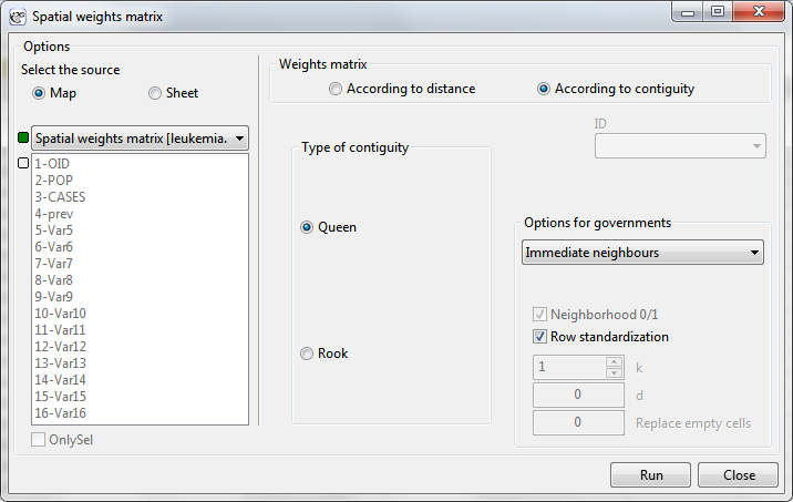
The objects neighborhood is defined by a spatial weight matrix. In Moran's analysis window we can choose any matrix generated previously by using menu Spatial analysis → Tools → Spatial weights matrix or indicate the neighbor matrix according to contiguity – Queen, row standardized, that is proposed by the program.

Note

It is not recommended to conduct Moran's analysis for objects without neighborhood (objects described in the weight matrix only with the 0 value). Such objects can be excluded from the analysis by deactivating them or an analysis can be made with the use of a different manner of defining neighborhood (a different weight matrix).

Moran's I coefficient – introduced by Moran in 1948 ¹⁾.

In order to check if the selected objects are characterized by similar values of the variable one can use the multiplying rule which says that multiplying 2 positive numbers gives a positive result and multiplying 2 different numbers (1 positive and 1 negative) gives a negative result. With the use of this rule we calculate $\sum\sum x_ix_j$ . Unfortunately, as the results of that rule are only obtained when there are both positive and negative values, the simple rule must be modified so as to ensure the presence of different signs. The values of the variable will, then, be replaced in the earlier formula with the differences of the values of the variable and of its mean value. In this way the objects with values smaller than the mean will be negative and those with values greater than the mean will be positive: $\sum\sum(x_i-\overline{x})(x_j-\overline{x})$ . Obviously, the summation should concern neighboring objects, which means that, at this point, information from weights matrices must be used:

$\begin{displaymath} \sum\sum w_{ij}(x_i-\overline{x})(x_j-\overline{x}) \end{displaymath}$

In this way non-neighboring objects obtain the weight value 0, for which reason the values of those objects are not added. Further operations which change the formula obtained in this manner are made with the view to making the obtained coefficient $I$ independent from the number of analyzed objects and to standardizing it so that its values are limited to the interval $<-1; 1>$ . As a result, Moran's autocorrelation coefficient is expressed with the formula:

$\begin{displaymath} I=\frac{\sum_{i=1}^n\sum_{j=1}^nw_{ij}\left(x_i-\overline{x}\right)\left(x_j-\overline{x}\right)}{S_0\sigma^2} \end{displaymath}$

where:

$n$ – the number of spatial objects (the number of points or polygons),

$x_i$ , $x_j$ – are the values of the variable for the compared objects,

$\overline{x}$ – it is the mean value of the variable for all objects,

$w_{ij}$ – elements of the spatial weights matrix (weights matrix row standardized),

$S_0=\sum_{i=1}^n\sum_{j=1}^nw_{ij}$ ,

$\sigma^2=\frac{\sum_{i=1}^n\left(x_i-\overline{x}\right)^2}{n}$ – variance

Moran's linear autocorrelation coefficient $I$ studies the strength of the linear relationship between the standardized variable $X$ ( $stand(x_i)$ ) and the spatial lag of the variable $X$ ( $L(x_i)$ ). Spatial lag is the weighted mean from the standardized values of neighboring objects

$\begin{displaymath} L(x_i)=\sum_{j=1}^Nw_{ij}stand(x_j). \end{displaymath}$

A graphic presentation of spatial autocorrelation is Moran's scatter plot. Points in the first quarter (HH) and in the third quarter (LL) are objects surrounded by similar neighbors: HH (high-high) – objects with high values, surrounded by objects with high values; LL (low-low) – objects with low values, surrounded by objects with low values. Points in the second quarter (LH) and the fourth quarter (HL) are objects surrounded by neighbors not similar to them. LH (low-high) – objects with low values, surrounded by objects with high values; HL (high-low) – objects with high values, surrounded by objects with low values.

$\begin{pspicture}(-4,-3.6)(10,4.5) \psline{->}(-4,0)(4,0) \psline{->}(0,-3.5)(0,4) \rput(1.5,1.5){\textcolor{red}{\textbf{\colorbox[rgb]{0.82,0.82,0.82}{HH}}}} \rput(-1.5,1.5){\textcolor[rgb]{0.2,0.8,0.8}{\textbf{\colorbox[rgb]{0.82,0.82,0.82}{LH}}}} \rput(-1.5,-1.5){\textcolor[rgb]{0,0,1}{\textbf{\colorbox[rgb]{0.82,0.82,0.82}{LL}}}} \rput(1.5,-1.5){\textcolor[rgb]{1,0.36,0.36}{\textbf{\colorbox[rgb]{0.82,0.82,0.82}{HL}}}} \psdot[dotsize=3pt](1.5,-0.6) \psdot[dotsize=3pt](0.8,0) \psdot[dotsize=3pt](1.1,0.2) \psdot[dotsize=3pt](2,-1.6) \psdot[dotsize=3pt](1.3,0) \psdot[dotsize=3pt](-1.6,1.9) \psdot[dotsize=3pt](-1.2,-1) \psdot[dotsize=3pt](1.3,0.5) \psdot[dotsize=3pt](1,0.6) \psdot[dotsize=3pt](0.2,-1.6) \psdot[dotsize=3pt](-0.6,0.2) \psdot[dotsize=3pt](-0.8,-1) \psdot[dotsize=3pt](1.9,0.7) \psdot[dotsize=3pt](1.8,-1.2) \psdot[dotsize=3pt](-1.8,-1) \psdot[dotsize=3pt](1.4,0.8) \psdot[dotsize=3pt](-0.6,-1.8) \psdot[dotsize=3pt](1.1,0.3) \psdot[dotsize=3pt](0.1,-1) \psdot[dotsize=3pt](-1.7,-1) \psdot[dotsize=3pt](1,-0.2) \psdot[dotsize=3pt](-0.4,-1.3) \psdot[dotsize=3pt](-1.1,-0.2) \psdot[dotsize=3pt](-0.1,-0.3) \psdot[dotsize=3pt](0.9,-0.9) \psdot[dotsize=3pt](-0.1,0.5) \psdot[dotsize=3pt](2,1.9) \psdot[dotsize=3pt](-1.5,-1) \psdot[dotsize=3pt](-1.5,1.1) \psdot[dotsize=3pt](0.6,-0.6) \psline[linewidth=1.8pt,linecolor=green](-2.5,-1)(2.5,1) \end{pspicture}$

The belonging to and distribution of points in the four quarters of Moran's diagram indicates the type of autocorrelation. If points are distributed mainly in the second quarter (LH) and fourth (HL) – it is a sign of negative correlation, if they belong mainly to the first quarter (HH) and third (LL) – it is a sign of positive correlation. If the points are distributed evenly in all four quarters then spatial autocorrelation does not exist.

On the Moran's diagram there is a regression line, the direction of which also allows to interpret Moran's coefficient $I$ :

$I>0$ indicates the presence of clusters of similar values – positive autocorrelation, i.e. measurement points lie near the straight line, and the increase of the variable $standX$ is reflected in the increase of the variable $L(X)$ ;
$I<0$ indicates the presence of the so-called hot spots, i.e. decidedly different values in neighboring areas – negative autocorrelation, i.e. measurement points lie near the straight line but the increase of the variable $standX$ is accompanied by a decrease of the variable $L(X)$ ;
$I \approx 0$ indicates random distribution of the studied value in space – a lack of autocorrelation, i.e. the obtained spatial distribution is as probable as any other distribution.

The square of Moran's coefficient $I^2$ informs about the degree (it is a percentage) to which the value of the variable in the object $i$ is explained by the value of that variable in neighboring objects.

Note

When the values of a studied feature are characterized by a great variability of variance then it is desirable to stabilize that variability. The basic information about smoothing variables have been described in the Chapter \ref{wygladz_przestrz} SPATIAL SMOOTHING

Significance of Moran's autocorrelation coefficient

A test for checking the significance of Moran's autocorrelation coefficient serves the purpose of verifying the hypothesis about a lack of correlation between $standX$ and spatial lag $L(X)$ .

Hypotheses:

$\begin{array}{cl} \mathcal{H}_0: & I = 0, \\ \mathcal{H}_1: & I \ne 0. \end{array}$

The test statistic has the form presented below:

$\begin{displaymath} Z=\frac{I-E(I)}{\sqrt{var(I)}}, \end{displaymath}$

where:

$\displaystyle E(I)=\frac{-1}{n-1}$ – the expected value,

$\displaystyle var(I)$ – variance.

Depending on the assumption concerning the distribution of the population from which the sample has been taken, the manner of selecting variance is chosen (Cliff and Ord (1981)²⁾, and Goodchild (1986)³⁾). If it is normal distribution, then:

$\begin{displaymath} var(I)=\frac{n^2S_1-nS_2+3S_0^2}{S_0^2(n^2-1)}-E(I)^2, \end{displaymath}$

where:

$S_1=\frac{1}{2}\sum_{i=1}^n\sum_{j=1}^n\left(w_{ij}+w_{ji}\right)^2$ ,

$S_2=\sum_{i=1}^n\left(\sum_{j=1}^nw_{ij}+\sum_{j=1}^nw_{ji}\right)^2$ .

If it is random distribution, then:

$\begin{displaymath} var(I)=\frac{n\left((n^2-3n+3)S_1-nS_2+3S_0^2\right)}{(n-1)^{(3)}S_0^2}-\frac{K_2\left((n^2-n)S_1-2nS_2+6S_0^2\right)}{(n-1)^{(3)}S_0^2}-E(I)^2, \end{displaymath}$

where:

$K_2=\frac{n\sum_{i=1}^n\left(x_i-\overline{x}\right)^4}{\left(\sum_{i=1}^n\left(x_i-\overline{x}\right)^2\right)^2}$ ,

$n^{(b)}=n(n-1)(n-2)...(n-b+1)$ .

Statistics asymptotically (for a large sample size) has the normal distribution.

The p-value, designated on the basis of the test statistic, is compared with the significance level $\alpha$ :

$\begin{array}{ccl} $ if $ p \le \alpha & \Longrightarrow & $ reject $ \mathcal{H}_0 $ and accept $ \mathcal{H}_1, \\ $ if $ p > \alpha & \Longrightarrow & $ there is no reason to reject $ \mathcal{H}_0. \\ \end{array}$

The window with settings for Moran's analysis is accessed via the menu Spacial statistics→Tools→Moran's global I statistic.

EXAMPLE (catalog: leukemia, file: leukemia.pqs)

The analysis will concern the data gathered and analyzed by L.A. Waller and others in 1992⁴⁾ and 1994⁵⁾, described on 281 objects in 2004⁶⁾.

The map leukemia contains information about the location of 281 polygons (census tracts) in the northern part of the state of New York. The map is prepared in the set of flat rectangular coordinate system UTM 18N and is based on the data of the file BNA (Boundary File) available on the server CIESIN ftp://ftp.ciesin.columbia.edu
Data for the map leukemia:
- Column CASES – the number of cases of leukemia in the years 1978-1982, ascribed to particular objects (census tracts). The value should be an integral number, however, in agreement with Waller's (1994) description, some cases which could not be objectively ascribed to a particular region have been divided proportionately. Hence, the numerousnesses of the cases ascribed to the 281 objects are not integral numbers.
- Column POP – population size in particular objects.
- Column prev – the frequency coefficient of leukemia per 100000 people, for each object in one year: prev=(CASES/POP)*100000/5

Epidemiologically interesting are the regions in which the prevalence of leukemia is higher, as their grouping could indicate the existence within their boundaries of environmental teratogens causing an increased frequency of occurrence of leukemia.

We start from presenting the geographic distribution of the frequency coefficient (prev) on the map. For that purpose we draw a map in the Map Manager and edit the layer , choosing Graduated colors:

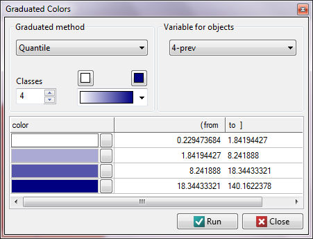
We have at our disposal several ways of coloring a map – we choose coloring in accordance with the values of the variable prev, dividing it into quartiles:

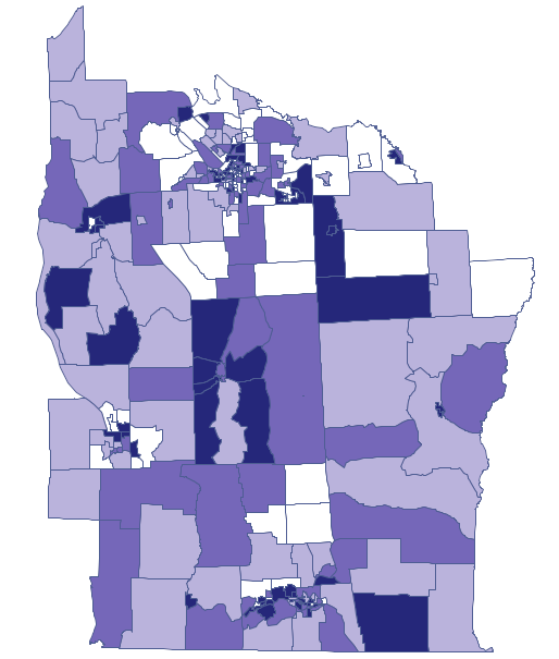
Dark colors on the map present the places with a higher frequency coefficient of leukemia, whereas light places signify a lower frequency coefficient. In order to learn if their geographic distribution is random or if they forms clusters, we will calculate Moran's coefficient. Before calculating that coefficient we should determine the manner of defining neighborhood of regions and it is advisable to create an appropriate weights matrix. In Moran's analysis window we can choose any matrix generated previously by using menu Spatial analysis → Tools → Spatial weights matrix or indicate the neighbor matrix according to contiguity – Queen, row standardized, that is proposed by the program.

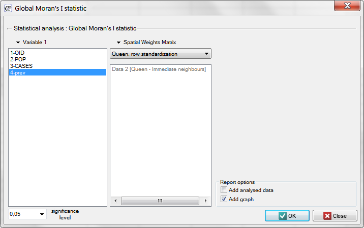
Having generated the weights matrix we select the file leukemia and start Moran's analysis by selecting the menu Spatial analysis → Spatial statistics → Global Moran's I statistic. In the analysis window we select the variable Prev and the neighbor matrix Queen, and select the option Add graph.

Moran's correlation coefficient obtained in the analysis is small and has the value $I=0.048577$ :

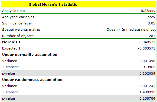
When we test the significance of Moran's coefficient we study the randomness of the distribution of the frequency coefficient of leukemia in the studied region. We check if similar shades on the map are located close to one another or not. In other words: we check if the odds of having leukemia in the studied population depends on geographic location or not. The value $p$ calculated with the assumption of randomness, as in the case of the assumption of normality, is greater than the standard assumed significance level 0.05, which means that there is no evidence for autocorrelation. Thus, we assume that the distribution of the variable prev is a random distribution. Moran's diagram confirms that assumption:

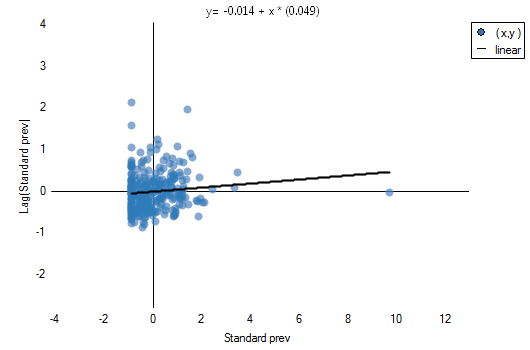
The existence of positive autocorrelation, in which we are the most interested, would result in the distribution of the points of the Moran's diagram in quarters I and III. Here, however, we see that the points are as frequent in quarters I and III as in II and IV.

2022/02/09 12:56

Global Geary's C statistic

Similarly to Moran's analysis, global Geary's statistic studies the degree of the intensity of a given feature in spatial objects.

Note

It is not recommended to conduct Geary's analysis for objects without a neighborhood (objects described in a weight matrix only with the value 0). Such objects can be excluded from the analysis by deactivating them (Chapter Limiting the workspace), or the analysis can be made with the use of a different manner of defining neighborhood (a different weight matrix).

Geary's autocorrelation coefficient – introduced by Geary in 1954 ⁷⁾.

It is one of the possible alternatives for the global Moran's statistic. Similarly to Moran's analysis, Geary's statistic studies the degree of intensity of a given $x_i$ feature in spatial objects described with the use of a weight matrix with $w_{ij}$ elements. This time, instead of computing the sum of quotients:

$\sum\sum w_{ij}(x_i-\overline{x})(x_j-\overline{x})$

we compute the sum of the difference squares:

$\begin{displaymath} \sum\sum w_{ij}(x_i-x_j)^2 \end{displaymath}$

As a result, Geary's autocorrelation coefficient is expressed with the formula:

$\begin{displaymath} c=\frac{\sum_{i=1}^n\sum_{j=1}^nw_{ij}(x_i-x_j)^2}{2 S_0 sd^2} \end{displaymath}$

where:

$n$ – the number of spatial objects (the number of points or polygons),

$x_i$ , $x_j$ – are the values of the variable for the compared objects,

$w_{ij}$ – elements of the spatial weights matrix (weights matrix row standardized),

$S_0=\sum_{i=1}^n\sum_{j=1}^nw_{ij}$ ,

$sd^2=\frac{\sum_{i=1}^n\left(x_i-\overline{x}\right)^2}{n-1}$ – variance,

$\overline{x}$ – it is the mean value of the variable for all objects.

The interpretation of Geary's coefficient:

$c<1$ and $c \approx 0$ means the occurrence of clusters with similar values – a positive autocorrelation;
$c>1$ means the occurrence of the so-called hot spots, i.e. distinctly different values in neighboring areas – a negative autocorrelation;
$c \approx 1$ means a random spatial distribution of the studied variable – a lack of autocorrelation.

Note

When the values of a studied feature are characterized by a great variability of variance then it is desirable to stabilize that variability. The basic information about smoothing variables have been described in the Chapter \ref{wygladz_przestrz} SPATIAL SMOOTHING

Significance of Geary's autocorrelation coefficient

A test for checking the significance of Geary's autocorrelation coefficient serves the purpose of verifying the hypothesis about a lack of spatial autocorrelation

Hypotheses:

$\begin{array}{cl} \mathcal{H}_0: & C = 1, \\ \mathcal{H}_1: & C \ne 1. \end{array}$

The test statistic has the form presented below:

$\begin{displaymath} Z=\frac{C-E(C)}{\sqrt{var(C)}}, \end{displaymath}$

where:

$\displaystyle E(C)=1$ – the expected value,

$\displaystyle var(C)$ – variance.

Depending on the assumption concerning the distribution of the population from which the sample has been taken, the manner of selecting variance is chosen (Cliff and Ord (1981)⁸⁾, and Goodchild (1986)⁹⁾). If it is a normal distribution, then:

$\begin{displaymath} var(C)=\frac{(2S_1+S_2)(n-1)-4S_0^2}{2(n+1)S_0^2}, \end{displaymath}$

where:

$S_1$ and $S_2$ are defined as for Moran's analysis.

If it is a random distribution, then:

$var(CS)=\frac{(n-1)S_1\left(n^2-3n+3-(n-1)b_2\right)-(n-1)S_2\left(n^2+3n-6-(n^2-n+2)b_2\right)\frac{1}{4}+S_0^2\left(n^2-3-(n-1)^2b_2\right)}{n(n-2)^{(2)}S_0^2},$

where:

$b_2=\frac{\frac{1}{n}\sum_{i=1}^n\left(x_i-\overline{x}\right)^4}{\left(\frac{1}{n}\sum_{i=1}^n\left(x_i-\overline{x}\right)^2\right)^2}$ ,

$n^{(b)}=n(n-1)(n-2)...(n-b+1)$ .

Statistics $Z$ has, asymptotically (for large sample sizes), normal distribution.

The p-value, designated on the basis of the test statistic, is compared with the significance level $\alpha$ :

$\begin{array}{ccl} $ if $ p \le \alpha & \Longrightarrow & $ reject $ \mathcal{H}_0 $ and accept $ \mathcal{H}_1, \\ $ if $ p > \alpha & \Longrightarrow & $ there is no reason to reject $ \mathcal{H}_0. \\ \end{array}$

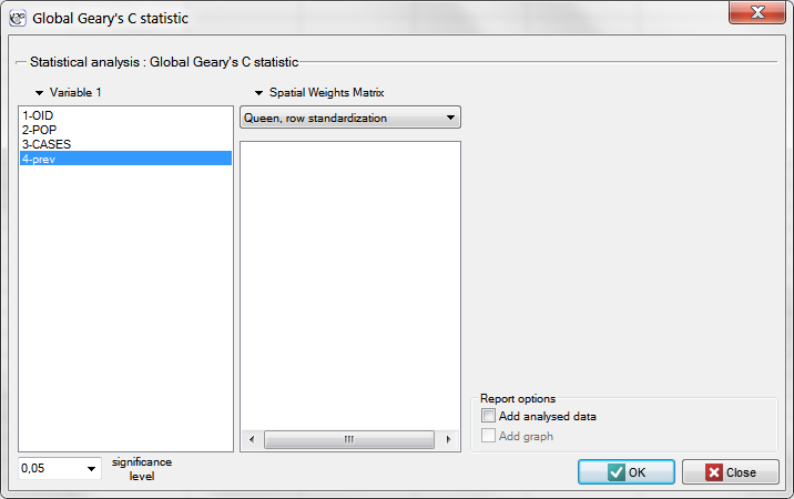
The window with settings for Geary's analysis is accessed via the men Spacial analysis → Spacial statistics → Global Geary's C statistic.

EXAMPLE cont. (catalog: leukemia, file: leukemia)

We will analyze the data concerning leukemia.

The map leukemia contains information about the location of 281 polygons (census tracts) in the northern part of the state of New York.
Data for the map leukemia:
- Column CASES – the number of cases of leukemia in the years 1978-1982, ascribed to particular objects (census tracts). The value should be an integral number, however, in agreement with Waller's (1994) description, some cases which could not be objectively ascribed to a particular region have been divided proportionately. Hence, the numerousnesses of the cases ascribed to the 281 objects are not integral numbers.
- Column POP – population size in particular objects.
- Column prev – the frequency coefficient of leukemia per 100000 people, for each object in one year: prev=(CASES/POP)*100000/5

Global Moran's analysis has pointed to a lack of spatial autocorrelation. This time, in order to check if in the studied area of the northern part of the state of New York it is possible to localize clusters of leukemia we will compute the global Geary's C statistic.

We start from the presentation of the geographic distribution of the prevalence coefficient (prev) on the map, according to the values of the prev variable, dividing it into quartiles:

Dark colors on the map present the places with a higher prevalence of leukemia, whereas light places signify a lower prevalence. Geary's correlation coefficient obtained in the analysis equals: 0.884986.

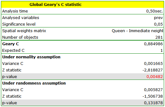
The obtained result, assuming a random distribution of data, is different from the result obtained with the assumption of a normal distribution. That can be indicative of an instability of the results and point to the need of further analyses based on smoothed variables.

2022/02/09 12:56

¹⁾

Moran P.A.P. (1947), The Interpretation of Statistical Maps. Journal of the Royal Statistical Society, B10, 243-51

²⁾ , ⁸⁾

Cliff A.D., Ord J.K. (1981), Spatial Processes: Models and Applications. Pion: London

³⁾

Goodchild M.F (1986), Spatial Autocorrelation, CATMOG 47, Geobooks: Norwich UK

⁴⁾

Waller L.A., Turnbull B.W., Clark L.C., Nasca P. (1992), Chronic disease surveillance and testing of clustering of disease and exposure : Application to leukemia incidence and TCE-contaminated dumpsites in upstate New York. Environmetrics, 3, 281-300

⁵⁾

Waller L.A., Turnbull B.W., Clark, L.C., Nasca P. (1994), Spatial pattern analyses to detect rare disease clusters, in Case Studies in Biometry, N. Lange, et al., Editors. , John Wiley and Sons: New York, 3-23

⁶⁾

Waller L.A., Gotway C.A. (2004), Applied Spatial Statistics for Public Health Data. New York: John Wiley and Sons

⁷⁾

Geary R.C. (1954), The Contiguity Ratio and Statistical Mapping. The Incorporated Statistician, 5, 115-45

⁹⁾

Goodchild M.F. (1986), Spatial Autocorrelation, CATMOG 47, Geobooks: Norwich UK

PQStat - Baza Wiedzy

Pasek boczny

Spis treści

Spatial autocorrelation

Global Moran's I statistic

Global Geary's C statistic

PQStat - Baza Wiedzy

Narzędzia użytkownika

Narzędzia witryny

Pasek boczny

Spis treści

Spatial autocorrelation

Global Moran's I statistic

Global Geary's C statistic

Narzędzia strony