PQStat - Baza Wiedzy

Spis treści

Density analysis
- Quadrat Count Methods
- Kernel density estimator
  - Two-dimensional kernel estimator
  - Three-dimensional kernel estimator

Density analysis

To conduct density analysis on the basis of a Map data we should have at our disposal a point, multipoint, or polygonal file. In the case of an analysis of a polygonal file, calculations are based on centroids of polygons, and in the case of a multipoint file they are based on centers of objects.

Quadrat Count Methods

Graphically, this method is a generalization of a histogram, or one-dimensional analysis, to a two-dimensional case. Building a histogram we have one variable, which we divide into intervals of equal length and give the number of cases in each interval. When building a grid of squares, we have two variables on which we build the grid and give the number of cases in each grid square (DPS – Dot Per Square). The ratio of this number to the area of a square determines the intensity of the color in which a given grid square is colored.

$\begin{tabular}{|l|l|l|l|} \hline \cellcolor[rgb]{0.8,0.8,0.8}&\textcolor[rgb]{1,1,1}{aaa}&\cellcolor[rgb]{0.4,0.4,0.4}\textcolor[rgb]{0.4,0.4,0.4}{aa}$\bullet$&\textcolor[rgb]{1,1,1}{aaa}\\ \cellcolor[rgb]{0.8,0.8,0.8}$\bullet$&&\cellcolor[rgb]{0.4,0.4,0.4}$\bullet$&\\ \hline \textcolor[rgb]{1,1,1}{aaa}&\textcolor[rgb]{1,1,1}{aaa}&\textcolor[rgb]{1,1,1}{aaa}&\textcolor[rgb]{0.8,0.8,0.8}{aa}\cellcolor[rgb]{0.8,0.8,0.8}$\bullet$\\ \textcolor[rgb]{1,1,1}{aaa}&\textcolor[rgb]{1,1,1}{aaa}&\textcolor[rgb]{1,1,1}{aaa}&\cellcolor[rgb]{0.8,0.8,0.8}\\ \hline \end{tabular}$

Based on the number of casess in the grid squares, we can study their spatial distribution. If there are the same number of points in each square, it means perfectly uniform distribution. When the opposite is true, when the variation in the number of points in the squares is very large, it means that there are squares with a much larger number of points, that is, clusters are formed.

If we denote by $n$ the number of points of the study area and by $m$ the number of squares into which the study area is divided, then we can determine the mean, variance, and standard deviation of the number of points per square:

$\begin{displaymath} \overline{DPS}=\frac{n}{m}, \quad Var_{(DPS)}=\frac{\sum_{i=1}^k m_i(n_i-\mu)^2}{m -1}, \quad SD_{(DPS)}=\sqrt{var}, \end{displaymath}$

where $m_i$ – is the number of squares with the number of points equal to $n_i$ .

Coefficient $VMR_{(DPS)}$

The most important information is provided by the variance-mean ratio – the coefficient, which is the quotient of the variance and the mean:

$\begin{displaymath} VMR_{(DPS)}=\frac{Var}{\overline{DPS}} \end{displaymath}$

A value of $VMR_{(DPS)}<1$ indicates too little variation in the number of points in squares which suggests a uniform dispersion effect, $VMR_{(DPS)}>1$ indicates too much variation in the number of points in squares and therefore a clustering effect, and a value close to 1 indicates an average variation in the number of points in squares which implies a random distribution of points.

The Index of Cluster Size (ICS) is often considered in the literature:

$\begin{displaymath} ICS_{(DPS)}=VMR_{(DPS)}-1 \end{displaymath}$ The expected value of $ICS_{(DPS)}$ assuming random points is 0. A positive value indicates a clustering effect and a negative value indicates a regular distribution of points.

Significance of the coefficient $VMR_{(DPS)}$

The $VMR_{(DPS)}$ coefficient significance test is used to verify the hypothesis that the observed point counts n the squares are the same as the expected counts that would occur for a random distribution of points.

Hypotheses:

$\begin{array}{ll} \mathcal{H}_0: & VMR_{(DPS)}=1,\\ \mathcal{H}_1: & VMR_{(DPS)} \neq 1. \end{array}$

The test statistic has the form:

$\begin{displaymath} \chi^2=(m-1)\cdot VMR_{(DPS)}. \end{displaymath}$

This statistic has an asymptotically $\chi^2$ distribution with $df=m-1$ degrees of freedom.

The p-value, designated on the basis of the test statistic, is compared with the significance level $\alpha$ :

$\begin{array}{ccl} $ if $ p \le \alpha & \Longrightarrow & $ reject $ \mathcal{H}_0 $ and accept $ \mathcal{H}_1, \\ $ if $ p > \alpha & \Longrightarrow & $ there is no reason to reject $ \mathcal{H}_0. \\ \end{array}$

Note

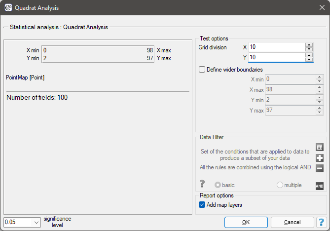
The result of the analysis depends to a large extent on the density of the grid and thus on the number/size of squares into which the analyzed area is divided. In the test options window, you can set the grid that will be used to divide the test area into squares by specifying the number of squares vertically and horizontally.

The window with the settings for the quadrat count method is launched via the menu Spatial Analysis→Spatial Statistics→Quadrat analysis

EXAMPLE (file squares.pqs)

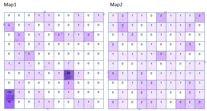
Using the datasheet, generate two point maps and perform a density analysis of these points. Answer the question: are the points randomly distributed in each of these maps?

You create the point maps using the formulas: menu Data→Formulas…

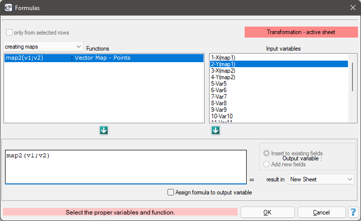
This will result in two new sheets containing maps. For each of these sheets, we perform a quadrat analysis.

Hypotheses:

$\begin{array}{ll} \mathcal{H}_0: & $the distribution of points in the population from which the sample is drawn is random ,$\\ \mathcal{H}_1: & $the distribution of points in the population from which the sample is drawn is not random.$ \end{array}$

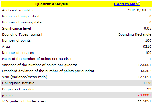
The results for Map 1 indicate a significant variation in the number of points in the squares, that is, a clustering effect (value p=<0.0001). This effect persists for different grid densities. For a grid density of 10:10 the VMR ratio is as high as 12.5, the entire report is included below:

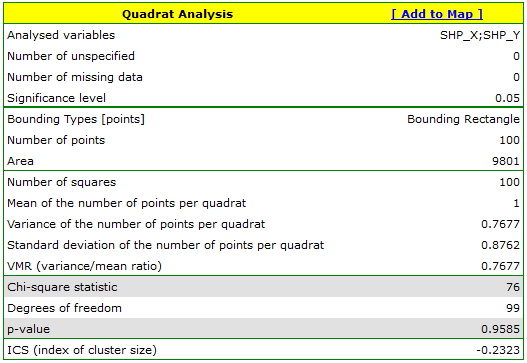
For map 2, the situation is quite different. For the 10:10 density grid, we have a lack of statistical significance (value p=0.9585) and the value of the coefficient VMR=0.77 indicate that the distribution of points is random.

Using the button in the report, we move to the Map Manager to select the analysis grid from the displayed list of layers and obtain a graphic interpretation of the results.

2022/02/09 12:56

Kernel density estimator

Two-dimensional kernel estimator

The two-dimensional kernel estimator (like the one-dimensional estimator) allows the distribution of the data, expressed by the method of squares, to be approximated by smoothing.

The two-dimensional kernel density estimator approximates the density of a data distribution by creating a smoothed density plane in a non-parametric manner. It produces a better density estimate than is given by the traditional method of squares, whose squares form a step function.

As in the one-dimensional case, this estimator is defined based on appropriately smoothed summed kernel functions (see description in the PQStat User Manual). There are several smoothing methods to choose from and several kernel functions described for the one-dimensional estimator (Gaussian, uniform, triangular, Epanechnikov, quartic/biweight). While the kernel function has little effect on the resulting plane smoothing, the smoothing factor does.

For each point $x$ in the range defined by the data, the density or kernel estimator is determined. It is obtained by summing the product of the kernel function values at that point:

$\begin{displaymath} \hat{f}_K(x,y)=\frac{1}{n}\sum_{i=1}^nK_h(t_i)K_h(s_i) \end{displaymath}$

If we give the individual cases weights $w_i$ , then we can construct a weighted nuclear density estimator defined by the formula:

$\begin{displaymath} \hat{f}_K(x,y)=\frac{1}{\sum_{i=1}^nw_i}\sum_{i=1}^nw_iK_h(t_i)K_h(s_i) \end{displaymath}$

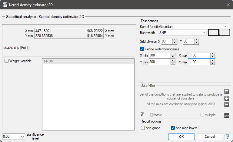
The window with settings for the kernel 2D density estimator ptions is launched via the menu Spatial analysis→Spatial statistics→Kernel density estimator 2D

EXAMPLE (snow.pqs plik)

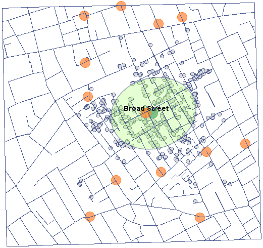
Currently, the main problem in presenting point data on the location of people is the need to protect them. Data protection prohibits publishing research results in such a way, that it would be possible to recognize a given person on their basis. A good solution in this case is a point density estimator.

We will present point data illustrating the cholera epidemic in London in 1854 using such an estimator. To do so, we will use a map of points (deaths due to cholera) with layers already overlaid to illustrate both streets and water pumps, and the result of an analysis by physician John Snow.

In the analysis window for the point map, we will stay with the Gaussian (normal) distribution kernel and the SNR smoothing factor. The grid density will be set to 80:80 and the boundaries will be increased so that the edges do not have a sharp edge by entering 300 as the minimum value for the X and Y coordinates and 1100 as the maximum value.

Using the 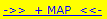button in the report, we go to the Map Manager, where we can add a layer representing this estimator (the last item in the list of layers).

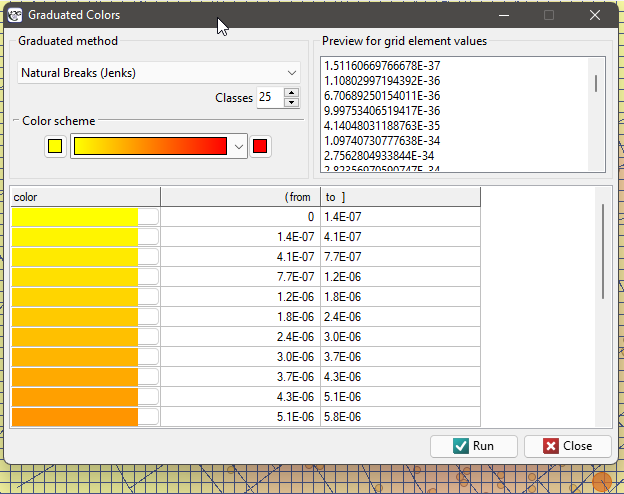
After applying the nuclear density estimator layer, edit it o remove the grid lines and change the yellow color to the natural background color (white in this case). The layer thus obtained is moved up g_kolejnosc_warstw, so that it is drawn at the beginning. We turn off the points layer (Base Map).

EXAMPLE cont. (squares.pqs file)

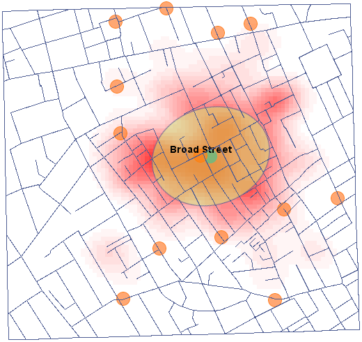
Using the kernel estimator, we represent the point density for map 1 - obtained in the earlier part of the task.

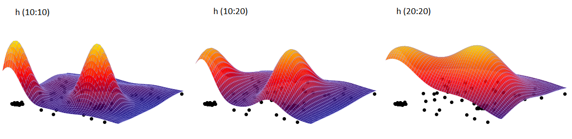
In the analysis window, we set the grid density to 50:50 and the kernel type as normal distribution and include a graph. We perform the analysis three times while changing the User smoothing factor: h (10:10), then h (10:20) and h (20:20). The obtained results presented on the map (via Map Manager) and on the 3D graph are shown below:

Three-dimensional kernel estimator

The three-dimensional kernel estimator (like the one-dimensional estimator and the two-dimensional estimator) allows you to approximate the distribution of the data by smoothing it.

The three-dimensional kernel density estimator approximates the density of the data distribution by creating a smoothed density plane in a non-parametric way. Graphically, we can represent it by plotting the first two dimensions in layers created by the third dimension. As in the one-dimensional case (see description in the PQStat User's Guide) and the two-dimensional estimator, this estimator is defined based on appropriately smoothed summed kernel functions. There are several smoothing methods to choose from and several kernel functions described for the one-dimensional estimator (Gaussian, uniform, triangular, Epanechnikov, quartic/biweight). While the kernel function has little effect on the resulting plane smoothing, the smoothing factor does.

For each point $x$ in the range defined by the data, the density that is the kernel estimator is determined. It is formed by summing the product of the kernel function values at that point:

$\begin{displaymath} \hat{f}_K(x,y,z)=\frac{1}{n}\sum_{i=1}^nK_h(t_i)K_h(s_i)K_h(r_i) \end{displaymath}$

If we give the individual cases weights $w_i$ , then we can construct a weighted kernel density estimator defined by the formula:

$\begin{displaymath} \hat{f}_K(x,y,z)=\frac{1}{\sum_{i=1}^nw_i}\sum_{i=1}^nw_iK_h(t_i)K_h(s_i)K_h(r_i) \end{displaymath}$

The window with settings for the kernel 3D density estimator options is launched via the menu Spatial analysis→Spatial statistics→Kernel 3D density estimator

Note

Displaying subsequent layers of the estimator, determined by the third dimension, is possible by editing the layer in the map Manager window and selecting the appropriate layer index.

2022/02/09 12:56

PQStat - Baza Wiedzy

Narzędzia użytkownika

Narzędzia witryny

Pasek boczny