PQStat - Baza Wiedzy

Spis treści

Kernel estimation
- One-dimensional kernel estimator

Kernel estimation

One-dimensional kernel estimator

The one-dimensional kernel density estimator allows you to approximate the density of a data distribution by creating a smoothed density curve in a non-parametric way. It provides a better density estimate than is given by a traditional histogram, which columns form a staircase function.

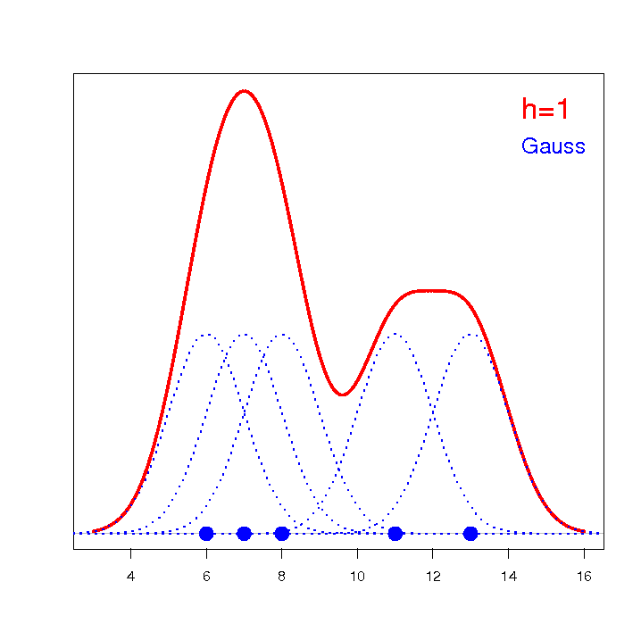
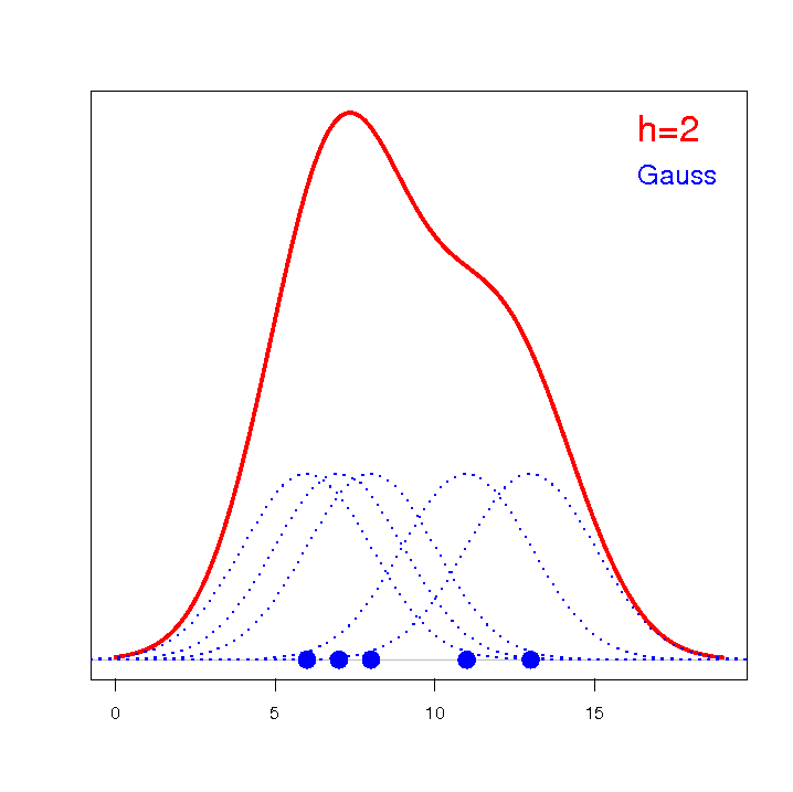
The kernel estimator is defined based on a properly smoothed kernel $K_h(t_i)$ . The smoothing parameter $h$ (bandwidth) has a decisive influence on the obtained estimator. The higher the value of the smoothing parameter, the greater the degree of smoothing.

For each point $x$ in the range defined by the data, the density is determined, that is, the value of the kernel estimator at that point is given. This estimator is created by summing the values of the kernel function $K_h(t_i)$ at that point:

$\begin{displaymath} \hat{f}_K(x)=\frac{1}{n}\sum_{i=1}^nK_h(t_i) \end{displaymath}$

If we give the individual cases weights $w_i$ , then we can construct a weighted kernel density estimator defined by the formula:

$\begin{displaymath} \hat{f}_K(x)=\frac{1}{\sum_{i=1}^nw_i}\sum_{i=1}^nw_iK_h(t_i) \end{displaymath}$

Smoothing factors

User - gives you the ability to select any user-specified smoothing factor, but the factor must be positive.
User scaled - is set so that the kernel function can be changed while remaining at the smoothing that was previously chosen for the Gauss kernel. In practice, by choosing a function other than Gauss, the smoothing factor is scaled (Scott, D. W. 1992¹⁾) so that the smoothing remains at a similar level as it was for the Gauss function. This offers the convenience of switching between different kernels without considering scaling the smoothing parameter. Scaling conversions are made based on the standard deviation:

$\begin{displaymath} h_2=\frac{\sigma(K_{h_1})}{\sigma(K_{h_2})}h_1 \end{displaymath}$

SNR - a smoothing factor constructed from Silverman's method (Silverman B. W. 1986 ²⁾ pp. 45 and 47) and Jones' correction (Jones M. C. et al 1996 ³⁾) using the standard deviation from the sample rather than the population - as proposed by Silverman:

$\begin{displaymath} h_{SNR}=1.06sd\cdot n^{1/5} \end{displaymath}$

For a non-Gaussian kernel, the smoothing factor is subject to scaling (Scott D. W., 1992⁴⁾)

SROT - smoothing factor built on the basis of Silverman's method (Silverman B. W. 1986 ⁵⁾ pp. 48) with Jones' correction (Jones M. C. i inni 1996⁶⁾):

$\begin{displaymath} h_{SROT}=0.9\min\left(sd, \frac{IQR}{1.34}\right) n^{1/5} \end{displaymath}$

For a non-Gaussian kernel, the smoothing factor is subject to scaling (Scott D. W., 1992⁷⁾)

OS - smoothing factor built on the basis of Terrell and Scott's method (Terrell G. R. i Scott D. W. 1985⁸⁾, Terrell G. R. 1990⁹⁾ pp. 470):

$\begin{displaymath} h_{OS}=1.144sd\cdot n^{1/5} \end{displaymath}$

For a non-Gaussian kernel, the smoothing factor is subject to scaling (Scott D. W., 1992¹⁰⁾)

Kernel function

The kernel function affects the obtained value of the kernel estimator to a lesser extent than the smoothing parameter. The kernel is a probability density function built around each data point $x_i$ . Typically, it is a symmetric function reaching a maximum at a point $x_i$ , and decreasing its values as one moves away (increasing distance $d_i$ ) from that point. The distance from the analysed point is modified by the smoothing parameter $h$ according to the formula: $t_i=\frac{d_i}{h}$ .

Depending on your needs, the kernel function can take the form of a function such as:

Gauss

$\begin{displaymath} K_h(t_i)=\frac{1}{h\sqrt{2\pi}}\exp(-\frac{t_i^2}{2}) \end{displaymath}$

uniform (rectanglular)

$\begin{displaymath} K_h(t_i)= \left\{ \begin{array}{ll} \frac{0,5}{h} & \textrm{if $t_i<1$}\\ 0 & \textrm{if $t_i \geq 1$}\\ \end{array} \right. \end{displaymath}$

triangular

$\begin{displaymath} K_h(t_i)= \left\{ \begin{array}{ll} \frac{1-t_i}{h} & \textrm{if $t_i<1$}\\ 0 & \textrm{if $t_i \geq 1$}\\ \end{array} \right. \end{displaymath}$

Epanechnikov

$\begin{displaymath} K_h(t_i)= \left\{ \begin{array}{ll} \frac{3}{4}\frac{1-t_i^2}{h} & \textrm{if $t_i<1$}\\ 0 & \textrm{if $t_i \geq 1$}\\ \end{array} \right. \end{displaymath}$

quartic or biweight (fourth degree)

$\begin{displaymath} K_h(t_i)= \left\{ \begin{array}{ll} \frac{15}{16}\frac{(1-t_i^2)^2}{h} & \textrm{ifi $t_i<1$}\\ 0 & \textrm{if $t_i \geq 1$}\\ \end{array} \right. \end{displaymath}$

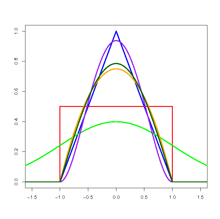
$\textcolor{green}{Gaussa} \textcolor{red}{uniform} \textcolor{blue}{triangular} \textcolor{orange}{Epanechnikova} \textcolor[rgb]{0,0.58,0}{quartic/biweight}$

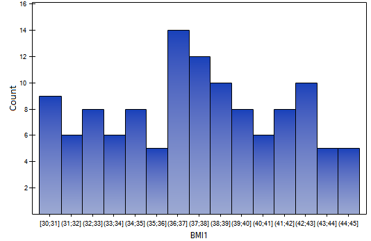
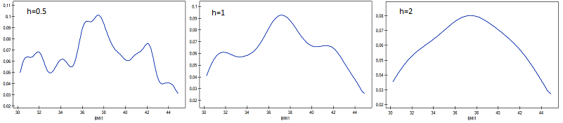
EXAMPLE (BMI.pqs file)

The values of the weight-growth index BMI1 for a certain group of obese subjects were calculated. Their distribution was presented using a histogram with the values divided every 1 BMI unit. The data were also visualized using a kernel density estimator by selecting a Gaussian kernel function and setting the smoothing factors to respectively: 0.5, 1, 2.

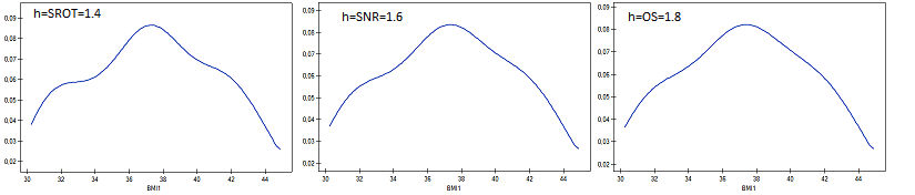
The smoothing factors of the kernel estimator suggested by the SROT, SNR, and OS methods reach magnitudes between 1.4 and 2.

¹⁾ , ⁴⁾ , ⁷⁾ , ¹⁰⁾

Scott D. W., (1992), Multivariate Density Estimation. Theory, Practice and Visualization. New York: Wiley

²⁾ , ⁵⁾

Silverman B. W., (1986), Density estimation for statistics and data analysis, London: Chapman and Hall

³⁾ , ⁶⁾

Jones M. C., Marron J. S., Sheather S. J., (1996)., A brief survey of bandwidth selection for density estimation. J. Amer. Statist. Assoc. 91 401–407

⁸⁾

Terrell G.R., Scott D. W. (1985), Oversmoothed nonparametric density estimates. Journal of the American Statistical Association 80, 209-214

⁹⁾

Terrell G. R. (1990), The maximal smoothing principle in density estimation. Journal of the American Statistical Association 85, 470–477

PQStat - Baza Wiedzy

Narzędzia użytkownika

Narzędzia witryny

Pasek boczny

Spis treści

Kernel estimation

One-dimensional kernel estimator

Narzędzia strony