Spis treści

Univariate MANOVA
- The univariate MANOVA

Univariate MANOVA

The univariate MANOVA

Beforehand, we recommend that you read the analysis of T-kwadrat Hotelling'a

Multivariate analysis of variance, is an extension of one-way ANOVA for independent groups. It is used to verify the hypothesis that the means of the $k$ variables under study are equal across several ( $m\geq2$ ) populations.

Staying with the ANOVA method involves comparing ( $m\geq2$ ) populations multiple times (separately for each variable) without taking into account the variables' correlation with each other. A MANOVA-type analysis, on the other hand, examines differences between populations one at a time for multiple variables, taking into account their correlation. In addition, the MANOVA approach is used as an alternative to the ANOVA for dependent groups because it does not require the sphericity assumption to be met.

Basic application conditions:

measurement on an interval scale,
A multivariate normal distribution in each population or normality of the distribution of each studied variable in each population,
independent model,
equality of the covariance matrix or equality of variances of the examined variables for the compared populations - a condition particularly important in the case of groups of different sizes.

Hypotheses:

$\begin{array}{cl} \mathcal{H}_0: & \mu_1=\mu_2=...=\mu_m,\\ \mathcal{H}_1: & $not all $\mu_i$ are equal,$ \end{array}$

where:

$\mu_i=(\mu_{i1}, \mu_{i2},..., \mu_{ik})$ - means of variables in $i$ -th population,

$(i=1,2,...,m)$ ,

$(j=1,2,...,k)$ .

We use several coefficients in MANOVA analyses. The most widely known is the Wilks' Lambda. The Pillai-Bartlett trace is the most conservative, but relatively robust to violations of the MANOVA assumptions and preferred for small sample sizes. The Hotelling-Lawley trace, on the other hand, is the least conservative of the three proposed tests. Work on the development of these techniques was begun by Wilks (1932)¹⁾, Pillai(1955)²⁾, Lawley(1938)³⁾, Hotelling(1951)⁴⁾, and Roy(1939)⁵⁾.

Test statistics are based on Sums of Squares and Cross Products ( $SSCP$ ) matrices. The total matrix $T=SSCP$ is broken down into two matrices, the first of which is related to the hypothesis being tested and is indicated by $H$ (in this case the matrix of between-group sums of squares and mixed products), and the second of which is related to the residuals (errors) and is indicated by $E$ (matrix of within-group sums of squares and mixed products).

Wilks' Lambda

Lambda value is defined as follows:

$\begin{displaymath} \Lambda=\frac{|E|}{|H+E|} \end{displaymath}$

The test statistic is in the form of:

$\begin{displaymath} F=\frac{1-\Lambda^{\frac{1}{b}}}{\Lambda^{\frac{1}{b}}}\frac{df_2}{df_1} \end{displaymath}$

where:

$df_1=k(m-1)$ , $df_2=ab-c$ ,

$a$ , $b$ , $c$ - coefficients dependent on the number of variables analyzed and the number of populations compared.

Hotelling-Lawley trail

The Hotelling-Lawley trace is defined as follows:

$\begin{displaymath} T_0=trace(HE^{-1}) \end{displaymath}$

The test statistic is in the form of:

$\begin{displaymath} F=\frac{T_0^2}{s}\frac{df_2}{df_1} \end{displaymath}$

where:

$df_1=s(2t+s+1)$ , $df_2=2(su+1)$ ,

$s$ , $t$ , $u$ - coefficients dependent on the number of variables analyzed and the number of populations compared.

Pillai-Bartlett trail

The Pillai-Bartlett trace is defined as follows:

$\begin{displaymath} V=trace(H(H+E)^{-1}) \end{displaymath}$

The test statistic is in the form of:

$\begin{displaymath} F=\frac{V}{s-V}\frac{df_2}{df_1} \end{displaymath}$

where:

$df_1=s(2t+s+1)$ , $df_2=s(2u+s+1)$ ,

$s$ , $t$ , $u$ - coefficients dependent on the number of variables analyzed and the number of populations compared.

Each of the test statistics above is subject to Snedecor's F distribution with $df_1$ and $df_2$ degrees of freedom.

The p-value, designated on the basis of the test statistic, is compared with the significance level $\alpha$ :

$\begin{array}{ccl} $ if $ p \le \alpha & \Longrightarrow & $ reject $ \mathcal{H}_0 $ and accept $ \mathcal{H}_1, \\ $ if $ p > \alpha & \Longrightarrow & $ there is no reason to reject $ \mathcal{H}_0. \\ \end{array}$

Effect size - partial <latex>$\eta^2$</latex>

This size indicates the proportion of explained variance to total variance associated with a given factor. In a one-factor MANOVA model for independent groups, it indicates what proportion of the within-group variability in outcomes can be attributed to the factor under study that determines the independent groups.

$\begin{displaymath} \eta^2=\frac{F\cdot df_1}{F\cdot df_1+df_2} \end{displaymath}$

Effect size - contrasts, one-dimensional analysis

When the analysis performed is to compare selected populations, or a selected set of populations, then we perform a contrasts analysis. This analysis is analogous to the contrasts in one-dimensional analysis but takes into account the interrelatedness of the variables.

For effect sizes, one can also determine simultaneous confidence intervals or confidence intervals with Bonferroni correction. When using these intervals, however, it is important to note that they do not take into account associations between variables (which MANOVA takes into account) but only multiple testing.

When looking for variables with differences, we can also use a one-dimensional approach. We then perform the comparisons of the ANOVA for independent groups separately for each variable. Unfortunately, this will not account for intercorrelations, but the p-values obtained from the ANOVA can be adjusted in the multiple comparisons section.

Note

The basic principle of MANOVA (as well as Hotelling's tests) is the construction of „multivariate ellipses” of confidence intervals around the centers determined by the means (see example interpretation of Hotelling's test ellipses for a single sample). As a result, using one-dimensional analysis (which does not take into account the interrelationships between variables) we are often unable to obtain identical results.

The settings window for the Single-factor MANOVA for independent groups is opened via menu Statistics→Parametric tests→MANOVA for independent groups.

EXAMPLE (sport.pqs file)

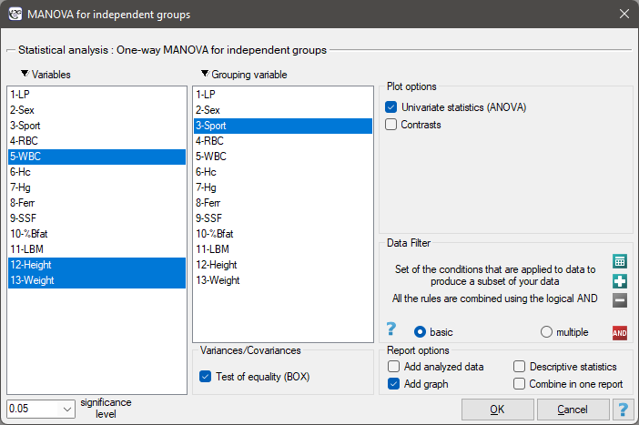
A group of athletes was studied to obtain information on health parameters such as:

WBC - White Blood Count,

Height [cm],

Body weight [kg].

We'd like to know:

Whether playing three types of sports professionally: „team games” (such as: basketball, volleyball, etc.) „running” (such as: 100m, 400m, etc.) „aquatic” (like: swimming, rowing, etc.), differ in the levels of these parameters.

Whether practicing high effort sports such as: „treadmill” and „aquatic” differ in the levels of these parameters from those practicing „team games”

[Re.1)]

Hypotheses:

$\begin{array}{cl} \mathcal{H}_0: & $The means of the analyzed parameters are the same $\\ & $for athletes participating in specific sports,$\\ \mathcal{H}_1: & $at least one parameter has a different mean value$\\ & $for the compared populations.$\\ \end{array}$

The result of Box's test (p=0.6302) allows us to calculate Analyses of the MANOVA type.

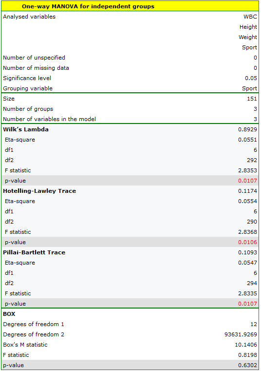
The significance of the coefficients: Wilks' Lambda, Hotelling-Lawley trace, and Pillai-Bartlett trace allow us to argue that the study populations of athletes differ on these parameters. To determine the differences we conduct a one-dimensional ANOVA analysis.

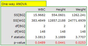
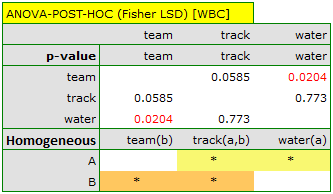
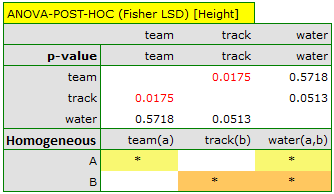
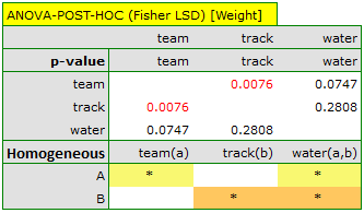
The results should be treated with caution. Although they indicate significant differences in all compared parameters, they yield p-values bordering on statistical significance (for WBC p=0.0489, for height p=0.0441, for weight p=0.0253). Additionally, when interpreting them, it is important to remember that they do not take into account either mutual correlation of parameters or multiple testing. Accounting for multiple testing in this case would require applying one of the p-value adjustments described in the section Multiple comparisons.

[Re.2)]

Hypotheses:

$\begin{array}{cl} \mathcal{H}_0: & $means of analyzed parameters for "team sports" $\\ & $are not different from the respective means of the athletes in the other two groups$\\ \mathcal{H}_1: & $at least one parameter has a different mean value$\\ & $for the compared populations.$\\ \end{array}$

To check whether the above hypotheses are true, we set an appropriate contrast in the analysis window. As a contrast value we enter 2 for team sports, -1 for treadmill and sports defined as aquatic.

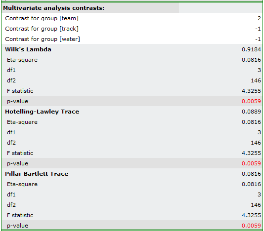
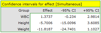
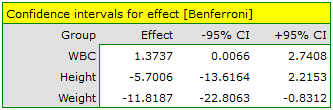
As a result, the obtained significance of the coefficients: Wilks' Lambda, Hotelling-Lawley trace and Pillai-Bartlett trace (p=0.0059) allows us to argue that athletes practicing high intensity sports differ in these parameters from those practicing team sports. In simultaneous intervals we do not observe these differences, while on the basis of Bonferroni intervals we can state that the difference concerns weight and WBC. WBC values are higher in the team sports group, and weight is significantly lower in this group.

2022/02/09 12:56

¹⁾

Wilks S.S. (1932), Certain generalizations in the analysis of variance. Biometrika 24: 471–494

²⁾

Pillai K. C. (1955), Some new test criteria in multivariate analysis. Annals of Mathematical Statistics 26: 117–121

³⁾

Lawley D. N. (1938), A generalization of Fisher’s z-test. Biometrika 30: 180–187.

⁴⁾

Hotelling H. (1951), A generalized t 2 test and measurement of multivariate dispersion. Proceedings of the Second Berkeley Symposium on Mathematical Statistics and Probability 1: 23–41

⁵⁾

Roy S. N. (1939), p-statistics or some generalizations in analysis of variance appropriate to multivariate problems. Sankhya 4: 381–396

PQStat - Baza Wiedzy

Pasek boczny

Spis treści

Univariate MANOVA

The univariate MANOVA

PQStat - Baza Wiedzy

Narzędzia użytkownika

Narzędzia witryny

Pasek boczny

Spis treści

Univariate MANOVA

The univariate MANOVA

Narzędzia strony