Spis treści

Descriptive statistics

Descriptive statistics

The purpose of using descriptive statistical methods is to summarize a set of data by certain characteristics, e.g., by the value of the mean, median, or standard deviation, and to draw some basic conclusions and generalizations about the dataset.

To calculate descriptive statistics for the data collected in the datasheet, open the Descriptive statistics window via menu Statistics→Descriptive analysis→Descriptive statistics.

In this window, we select the variable to be analysed and the analysis settings and select the descriptive statistics measures we are interested in. You may select individual statistics or groups of statistics by clicking on the . Confirm the selection by pressing OK. The result of the analysis will be in a report attached to the datasheet for which the analysis was performed.

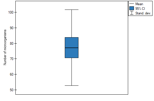
In addition, if you want the data to be visualized with a box-and-whisker chart, then in the Descriptive statistics window select the Add graph.

Location measures

Measures of central tendency

Measures of central tendency are so-called average measures that characterize the average or typical level of a trait's values.

Arithmetic mean is expressed by the formula: $\begin{displaymath} \overline{x}=\frac{x_1+x_2+\cdots+x_n}{n}=\frac{\sum_{i=1}^{n}x_i}{n}, \end{displaymath}$

where $x_i$ is the consecutive values of the variable and $n$ is the sample size.

The arithmetic mean is used for interval scale. For a sample it is taken to be denoted by $\overline{x}$ and for a population by $\mu$ .

Trimmed mean - is determined as the arithmetic mean calculated after removing from the sample a given percentage of the smallest and largest measurements, e.g. if we cut off 5 per cent of the measurements, it means that we cut off 2.5 per cent of the largest and 2.5 per cent of the smallest values. At the same time, if the number of measurements to be removed obtained from the conversion is not an integer, it is rounded down to the nearest whole number.

Winsor mean - is determined as the arithmetic mean calculated after replacing the appropriate percentage of extreme measurements with the smallest and largest value that remains of the reduced set of values. If we choose to calculate the Winsor average by pruning, say, 5% of the measurements, then those discarded 5% will be replaced by the smallest and largest value determined from the remaining 95% of the measurements. As with the pruned average, when converting the percentage of values to be replaced to the number of measurements to be replaced does not result in an integer, then we round down to the nearest integer. Geometric mean is expressed by the formula: $\begin{displaymath} \overline{x}_G=\sqrt[n]{x_1x_2...x_n}=\sqrt[n]{\prod_{i=1}^n x_i}. \end{displaymath}$ This mean is used for the interval scale, when the variable has a log-normal distribution (the logarithm of the variable has a normal distribution).

Harmonic mean is expressed by the formula: $\begin{displaymath} \overline{x}_H=\frac{n}{\frac{1}{x_1}+\frac{1}{x_2}+\cdots+\frac{1}{x_n}}=\frac{n}{\sum_{i=1}^{n}\frac{1}{x_i}}. \end{displaymath}$ This mean is used for the interval scale.

Median

In an ordered data set, the median is the value that divides the data set into two equal parts. Half of all observations are below and half are above the median.

$\begin{pspicture}(0,0)(3,4.6) \pscoil[coilaspect=0, coilarm=.1cm, linewidth=0.5pt, coilwidth=.5cm, coilheight=1]{-}(0,4) \rput(0,4.2){min} \rput(0,-.2){max} \psline(-0.35,2)(.35,2) \rput(1.2,2){median} \rput(-0.6,2.8){50$\%$} \rput(-0.6,1.2){50$\%$} \end{pspicture}$

The median can be used in interval and ordinal scale.

Mode

Mode $-$ is the value that occurs most frequently among the measurements obtained. Fashion can be used at any measurement scale.

2022/02/09 12:56

Other measures of location

Quartiles, deciles, centiles

$\begin{pspicture}(0,-.2)(4,4.4) \pscoil[coilaspect=0, coilarm=.1cm, linewidth=0.5pt, coilwidth=.5cm, coilheight=1]{-}(0,4) \rput(0,4.2){max} \rput(0,-.2){min} \psline(-0.35,3)(.35,3) \psline(-0.35,2)(.35,2) \psline(-0.35,1)(.35,1) \rput(2.9,3){$C_{75}$ = upper quartile = $Q_3$} \rput(2.4,2){$C_{50}$ = median = $Q_2$} \rput(2.9,1){$C_{25}$ = lower quartile = $Q_1$} \rput(1,3.5){25$\%$} \rput(1,2.5){25$\%$} \rput(1,1.5){25$\%$} \rput(1,.5){25$\%$} \end{pspicture}$

Quartiles ( $Q_1$ , $Q_2$ , $Q_3$ ) divide the ordered series into 4 equal parts, deciles ( $D_i$ , $i=1,2,...,9$ ) into 10 equal parts and centiles (percentiles: $C_i$ , $i=1,2,...,99$ ) into 100 equal parts. The second quartile, fifth decile, and fiftieth centile are equal to the median. These measures can be used in the interval and ordinal scale.

2022/02/09 12:56

Measures of variability (dispersion)

Central tendency measures knowledge is not enough to fully describe a statistical data collection structure. The researched groups may have various variation levels of a feature you want to analyse. You need some formulas then, which enable you to calculate values of variability of the features.

Measures of variability are calculated only for an interval scale, because they are based on the distance between the points.

Range is formulated:

$\begin{displaymath} I=\max x_i - \min x_i \label{rozstep}, \end{displaymath}$

where $x_i$ are values of the analysed variable

$\begin{displaymath} IQR=\textrm{Interquartile range}=Q_3-Q_1 \label{rozstepkw}, \end{displaymath}$

where $Q_1, Q_3$ are the lower and the upper quartile.

Ranges for a percentile scale (decile, centile) Ranges between percentiles are one of the dispersion measures. They define a percentage of all observations, which are located between the chosen percentiles.

Variance $-$ measures a degree of spread of the measurements around arithmetic mean

sample variance:

$\begin{displaymath} sd^2=\displaystyle{\frac{\sum_{i=1}^{n}(x_i-\overline{x})^2}{n-1}}, \label{wariancja} \end{displaymath}$

where $x_i$ are following values of variable and $\overline{x}$ is an arithmetic mean of these values, n - sample size;

population variance:

$\begin{displaymath} \sigma^2=\displaystyle{\frac{\sum_{i=1}^{N}(x_i-\mu)^2}{N}}, \label{wariancja} \end{displaymath}$

where $x_i$ are following values of variables and $\mu$ is an arithmetic mean of these values, $N$ - population size;

Variance is always positive, but it is not expressed in the same units as measuring results.

Standard deviation $-$ measures a degree of spread of the measurements around arithmetic mean.

sample standard deviation:

$\begin{displaymath} sd=\sqrt{sd^2}, \label{odch.standard} \end{displaymath}$

population standard deviation:

$\begin{displaymath} \sigma=\sqrt{\sigma^2}. \end{displaymath}$

The higher standard deviation or a variance value is, the more diversed is the group in relation to an analysed feature.

Note The sample standard deviation is a kind of approximation (estimator) of the population standard deviation. The population standard deviation value is included in a range which contains the sample standard deviation. This range is called a **confidence interval ** for standard deviation.

Coefficient of variation

Coefficient of variation, just like standard deviation, enables you to estimate the homogeneity level of an analysed data collection. It is formulated as:

$\begin{displaymath} V=\frac{sd}{\overline{x}}100\% , \label{wspzmienn} \end{displaymath}$

where $sd$ means standard deviation, $\overline{x}$ means arithmetic mean.

This is a unitless value. It enables you to compare a diversity of several different datasets of a one feature. And also, you are able to compare a diversity of several features (expressed in different units). It is assumed, if $V$ coefficient does not exceed 10%, features indicate a statistically insignificant diversity.

Standard errors $-$ they are not measures of a measurement dispersion. They measure an accuracy level, you can define the population parameters value, having just the sample estimators.

Standard error of the mean is defined by:

$\begin{displaymath} SEM=\textrm{standard error of the mean}=\frac{sd}{\sqrt{n}} \label{sem}. \end{displaymath}$

Note

On the basis of a sample estimator you can calculate a confidence interval for a population parameter.

2022/02/09 12:56

Another distribution characteristics

Skewness or asymmetry coefficient in other words

This measure tells us how data distribution differs from symmetrical distribution. The closer the value of skewness is to zero, the more symmetrically around the mean the data are spread. Usually the value of this coefficient is included in a range [-1, 1], but in the case of a very big asymmetry, it may occur outside the above-mentioned range. A positive skew value indicates that the right skew occurs (the tail on the right side is longer), whereas the negative skew indicates that the left skew occurs (the tail on the left side is longer). Skewness is defined by:

$\begin{displaymath} A=\frac{n}{(n-1)(n-2)}\sum_{i=1}^n\left(\frac{x_i-\overline{x}}{sd}\right)^3, \end{displaymath}$

where:

$x_i$ $-$ the following values of a variable,

$\overline{x}$ , $sd$ $-$ adequately - arithmetic mean and standard deviation $x_i$ ,

$n$ $-$ sample size.

$\begin{tabular}{cc} \begin{pspicture}(0,-.7)(7,3.6) \rput(2.5,3.3){right skew} \rput(2.8,2.8){$A>0$} \psline{->}(0,0)(0,3) \psline{->}(0,0)(6.3,0) \psbezier{-}(.2,.2)(.5,.2)(.7,2.3)(1.3,2.5) \psbezier{-}(1.3,2.5)(2,2.5)(3,.2)(5.3,.2) \psline[linestyle=dotted]{-}(2.2,0)(2.2,1.7) \rput(2.55,-.3){Med.} \psline[linestyle=dotted]{-}(1.3,0)(1.3,2.5) \rput(1.3,-.3){Mode} \psline[linestyle=dotted]{-}(3.4,0)(3.4,.7) \rput(3.5,-.3){$\overline{X}$} \rput{90}(-.4,2.7){frequency} \rput(6.1,-.3){x} \end{pspicture} & \begin{pspicture}(0,-.7)(7,3.6) \rput(2.5,3.3){left skew} \rput(2.2,2.8){$A<0$} \psline{->}(0,0)(0,3) \psline{->}(0,0)(6.3,0) \psbezier{-}(.2,.2)(2.1,.2)(2.8,2.5)(3.7,2.5) \psbezier{-}(3.7,2.5)(4.2,2.5)(4.8,.2)(5.5,.2) \psline[linestyle=dotted]{-}(2.85,0)(2.85,1.75) \rput(2.7,-.3){Med.} \psline[linestyle=dotted]{-}(3.7,0)(3.7,2.5) \rput(3.9,-.3){Mode} \psline[linestyle=dotted]{-}(1.7,0)(1.7,.7) \rput(1.7,-.3){$\overline{X}$} \rput{90}(-.4,2.7){frequency} \rput(6.1,-.3){x} \end{pspicture} \end{tabular}$

Kurtosis or coefficient of concentration

This measure tells us how much the spread of data around the mean is similar to the spread of data in normal distribution. The greater than zero the value of kurtosis is, the more narrow the tested distribution than normal one is. And inversely, the lower than zero the value of kurtosis is, the flatter the tested distribution than the normal one is. Kurtosis is defined by:

$\begin{displaymath} K=\frac{n(n+1)}{(n-1)(n-2)(n-3)}\sum_{i=1}^n\left(\frac{x_i-\overline{x}}{sd}\right)^4-\frac{3(n-1)^2}{(n-2)(n-3)}, \end{displaymath}$

where:

$x_i$ $-$ the following values of a variable,

$\overline{x}$ , $sd$ $-$ adequately - arithmetic mean and standard deviation of $x_i$ ,

$n$ $-$ sample size.

$\begin{pspicture}(0,-.8)(6.5,3.4) \rput(4.0,.7){$K_1<0$} \rput(4.5,2.5){$K_2>0$} \psline{->}(0,0)(0,3) \psline{->}(0,0)(7,0) \psbezier[linestyle=dashed]{-}(.2,.2)(2.2,.8)(2.3,1.4)(3.2,1.5) \psbezier[linestyle=dashed]{-}(3.2,1.5)(4.1,1.4)(4.2,.8)(6.2,.2) \psbezier{-}(.4,.2)(2.4,.6)(2.5,3.0)(3.2,3.1) \psbezier{-}(3.2,3.1)(3.9,3.0)(4.0,.6)(6.0,.2) \psline[linestyle=dotted]{-}(3.2,0)(3.2,3.1) \rput(3.2,-.3){$\overline{X}$} \rput{90}(-.4,2.7){frequency} \rput(6.8,-.3){x} \end{pspicture}$

EXAMPLE (fertilisers.pqs file)

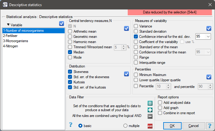
In an experiment related to a soil fertilising the with various sorts of microbiological specimens and fertilisers it was calculated how many microorganisms occur in a 1 gramme of dry mass of soil. Now we would like to calculate descriptive statistics of the amount of actinomycetes for the sample fertilised with nitrogen. Additionally, we want the data to be illustrated in the Box-Whiskers plot. In a datasheet, we select only the 54 first rows, which are relevant to the assumptions of the analysis (there are actinomycetes fertilised with nitrogen). Then we open Descriptive statistics window in Statistics menu→Descriptive analysis→Descriptive statistics.

In the window of descriptive statistics options, select a variable to analyse: the number of microorganisms, and then all the procedures you want to follow (for example arithmetic mean altogether with the confidence interval, median, standard deviation altogether with the confidence interval, and an information about the skewness and kurtosis of distribution altogether with errors). At the top of the window you should see the following message:

Data limited by the selected area

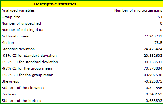
. To add a graph to the report, we select Add graph option and chose the Box-Whiskers plot type. Confirm your choice by clicking OK and you get the result in a report:

2022/02/09 12:56

PQStat - Baza Wiedzy

Pasek boczny

Spis treści

Descriptive statistics

Location measures

Measures of central tendency

Other measures of location

Measures of variability (dispersion)

Another distribution characteristics

PQStat - Baza Wiedzy

Narzędzia użytkownika

Narzędzia witryny

Pasek boczny

Spis treści

Descriptive statistics

Location measures

Measures of central tendency

Other measures of location

Measures of variability (dispersion)

Another distribution characteristics

Narzędzia strony