PQStat - Baza Wiedzy

The ANOVA for independent groups

The one-way analysis of variance (ANOVA for independent groups) proposed by Ronald Fisher, is used to verify the hypothesis determining the equality of means of an analysed variable in several ( $k\geq2$ ) populations.

Basic assumptions:

measurement on an interval scale,
normality of distribution of an analysed feature in each population,
an independent model,
equality of variances of an analysed variable in all populations.

Hypotheses:

$\begin{array}{cl} \mathcal{H}_0: & \mu_1=\mu_2=...=\mu_k,\\ \mathcal{H}_1: & $not all $\mu_j$ are equal $(j=1,2,...,k)$,$ \end{array}$

where:

$\mu_1$ , $\mu_2$ ,…, $\mu_k$ – means of an analysed variable of each population.

The test statistic is defined by:

$\begin{displaymath} F=\frac{MS_{BG}}{MS_{WG}}, \end{displaymath}$

where:

$\displaystyle MS_{BG} = \frac{SS_{BG}}{df_{BG}}$ – mean square between-groups,

$\displaystyle MS_{WG} = \frac{SS_{WG}}{df_{WG}}$ – mean square within-groups,

$\displaystyle SS_{BG} = \sum_{j=1}^k{\frac{\left(\sum_{i=1}^{n_j}x_{ij}\right)^2}{n_j}}-\frac{\left(\sum_{j=1}^k{\sum_{i=1}^{n_j}x_{ij}}\right)^2}{N}$ – between-groups sum of squares,

$\displaystyle SS_{WG} = SS_{T}-SS_{BG}$ – within-groups sum of squares,

$\displaystyle SS_{T} = \left(\sum_{j=1}^k{\sum_{i=1}^{n_j}x_{ij}^2}\right)-\frac{\left(\sum_{j=1}^k{\sum_{i=1}^{n_j}x_{ij}}\right)^2}{N}$ – total sum of squares,

$df_{BG}=k-1$ – between-groups degrees of freedom,

$df_{WG}=df_{T}-df_{BG}$ – within-groups degrees of freedom,

$df_{T}=N-1$ – total degrees of freedom,

$N=\sum_{j=1}^k n_j$ ,

$n_j$ – samples sizes for $(j=1,2,...k)$ ,

$x_{ij}$ – values of a variable taken from a sample for $(i=1,2,...n_j)$ , $(j=1,2,...k)$ .

The F statistic has the F Snedecor distribution with $df_{BG}$ and $df_{WG}$ degrees of freedom.

The p-value, designated on the basis of the test statistic, is compared with the significance level $\alpha$ :

$\begin{array}{ccl} $ if $ p \le \alpha & \Longrightarrow & $ reject $ \mathcal{H}_0 $ and accept $ \mathcal{H}_1, \\ $ if $ p > \alpha & \Longrightarrow & $ there is no reason to reject $ \mathcal{H}_0. \\ \end{array}$

Effect size - partial $\eta^2$

This quantity indicates the proportion of explained variance to total variance associated with a factor. Thus, in a one-factor ANOVA model for independent groups, it indicates what proportion of the between-groups variability in outcomes can be attributed to the factor under study determining the independent groups.

$\begin{displaymath} \eta^2=\frac{SS_{BG}}{SS_{BG}+SS_{res}} \end{displaymath}$

POST-HOC tests

Introduction to contrast and POST-HOC testing

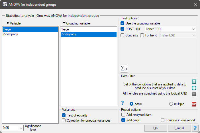
The settings window with the One-way ANOVA for independent groups can be opened in Statistics menu→Parametric tests→ANOVA for independent groups or in ''Wizard''.

EXAMPLE(age ANOVA.pqs file)

There are 150 persons chosen randomly from the population of workers of 3 different transport companies. From each company there are 50 persons drawn to the sample. Before the experiment begins, you should check if the average age of the workers of these companies is similar, because the next step of the experiment depends on it. The age of each participant is written in years. Age (company 1): 27, 33, 25, 32, 34, 38, 31, 34, 20, 30, 30, 27, 34, 32, 33, 25, 40, 35, 29, 20, 18, 28, 26, 22, 24, 24, 25, 28, 32, 32, 33, 32, 34, 27, 34, 27, 35, 28, 35, 34, 28, 29, 38, 26, 36, 31, 25, 35, 41, 37\\Age (company 2): 38, 34, 33, 27, 36, 20, 37, 40, 27, 26, 40, 44, 36, 32, 26, 34, 27, 31, 36, 36, 25, 40, 27, 30, 36, 29, 32, 41, 49, 24, 36, 38, 18, 33, 30, 28, 27, 26, 42, 34, 24, 32, 36, 30, 37, 34, 33, 30, 44, 29\\Age (company 3): 34, 36, 31, 37, 45, 39, 36, 34, 39, 27, 35, 33, 36, 28, 38, 25, 29, 26, 45, 28, 27, 32, 33, 30, 39, 40, 36, 33, 28, 32, 36, 39, 32, 39, 37, 35, 44, 34, 21, 42, 40, 32, 30, 23, 32, 34, 27, 39, 37, 35.

Before proceeding with the ANOVA analysis, the normality of the data distribution was confirmed.

The analysis window tested the assumption of equality of variance, obtaining p>0.05 in both tests.

Hypotheses:

$\begin{array}{cl} \mathcal{H}_0: & $the average age of the workers off all the analysed transport companies is the same,$\\ \mathcal{H}_1: & $at least 2 means are different.$ \end{array}$

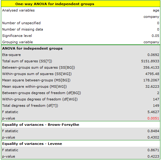
Comparing the p-value = 0.005147 of the one-way analysis of variance with the significance level $\alpha=0.05$ , you can draw the conclusion that the average ages of workers of these transport companies is not the same. Based just on the ANOVA result, you do not know precisely which groups differ from others in terms of age. To gain such knowledge, it must be used one of the POST-HOC tests, for example the Tukey test. To do this, you should resume the analysis by clicking and then, in the options window for the test, you should select Tukey HSD and Add graph.

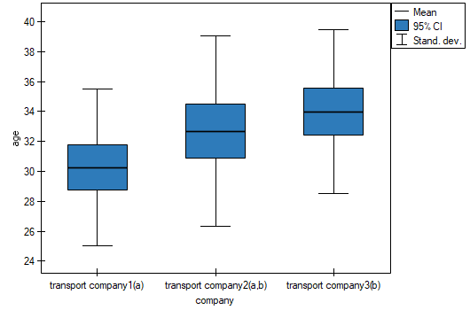
The critical difference (CD) calculated for each pair of comparisons is the same (because the groups sizes are equal) and counts to 2.730855. The comparison of the $CD$ value with the value of the mean difference indicates, that there are significant differences only between the mean age of the workers from the first and the third transport company (only if these 2 groups are compared, the $CD$ value is less than the difference of the means). The same conclusion you draw, if you compare the p-value of POST-HOC test with the significance level $\alpha=0.05$ . The workers of the first transport company are about 3 years younger (on average) than the workers of the third transport company. Two interlocking homogeneous groups were obtained, which are also marked on the graph.

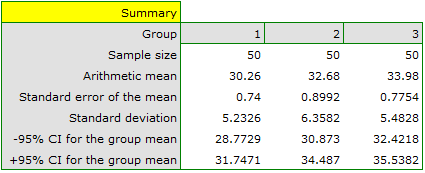
We can provide a detailed description of the data by selecting Descriptive statistics in the analysis window

PQStat - Baza Wiedzy

Narzędzia użytkownika

Narzędzia witryny

Pasek boczny

The ANOVA for independent groups

Narzędzia strony