Narzędzia użytkownika
Narzędzia witryny
Pasek boczny
en:statpqpl:porown3grpl:parpl
Spis treści
Parametric tests
The ANOVA for independent groups
The one-way analysis of variance (ANOVA for independent groups) proposed by Ronald Fisher, is used to verify the hypothesis determining the equality of means of an analysed variable in several ( ) populations.
Basic assumptions:
- measurement on an interval scale,
- normality of distribution of an analysed feature in each population,
- equality of variances of an analysed variable in all populations.
Hypotheses:

where:
 ,
, ,…,
,…, – means of an analysed variable of each population.
The test statistic is defined by:

where:
 – mean square between-groups,
 – mean square within-groups,
 – between-groups sum of squares,
 – within-groups sum of squares,
 – total sum of squares,
 – between-groups degrees of freedom,
 – within-groups degrees of freedom,
 – total degrees of freedom,
 ,
,
 – samples sizes for
  ,
,
 – values of a variable taken from a sample for
  , .
, .
The F statistic has the F Snedecor distribution with  and
and  degrees of freedom.
The p-value, designated on the basis of the test statistic, is compared with the significance level  :
:

Effect size - partial 
This quantity indicates the proportion of explained variance to total variance associated with a factor. Thus, in a one-factor ANOVA model for independent groups, it indicates what proportion of the between-groups variability in outcomes can be attributed to the factor under study determining the independent groups.

POST-HOC tests
Introduction to contrast and POST-HOC testing
The settings window with the One-way ANOVA for independent groups can be opened in Statistics menu→Parametric tests→ANOVA for independent groups or in ''Wizard''.
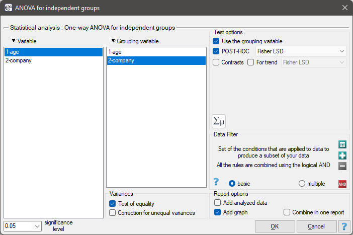
There are 150 persons chosen randomly from the population of workers of 3 different transport companies. From each company there are 50 persons drawn to the sample. Before the experiment begins, you should check if the average age of the workers of these companies is similar, because the next step of the experiment depends on it. The age of each participant is written in years.
Age (company 1): 27, 33, 25, 32, 34, 38, 31, 34, 20, 30, 30, 27, 34, 32, 33, 25, 40, 35, 29, 20, 18, 28, 26, 22, 24, 24, 25, 28, 32, 32, 33, 32, 34, 27, 34, 27, 35, 28, 35, 34, 28, 29, 38, 26, 36, 31, 25, 35, 41, 37\\Age (company 2): 38, 34, 33, 27, 36, 20, 37, 40, 27, 26, 40, 44, 36, 32, 26, 34, 27, 31, 36, 36, 25, 40, 27, 30, 36, 29, 32, 41, 49, 24, 36, 38, 18, 33, 30, 28, 27, 26, 42, 34, 24, 32, 36, 30, 37, 34, 33, 30, 44, 29\\Age (company 3): 34, 36, 31, 37, 45, 39, 36, 34, 39, 27, 35, 33, 36, 28, 38, 25, 29, 26, 45, 28, 27, 32, 33, 30, 39, 40, 36, 33, 28, 32, 36, 39, 32, 39, 37, 35, 44, 34, 21, 42, 40, 32, 30, 23, 32, 34, 27, 39, 37, 35.
Before proceeding with the ANOVA analysis, the normality of the data distribution was confirmed.
The analysis window tested the assumption of equality of variance, obtaining p>0.05 in both tests.
Hypotheses:

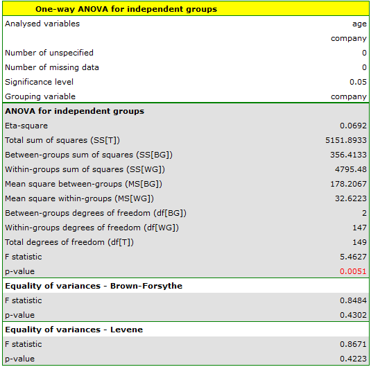
Comparing the p-value = 0.005147 of the one-way analysis of variance with the significance level  , you can draw the conclusion that the average ages of workers of these transport companies is not the same. Based just on the ANOVA result, you do not know precisely which groups differ from others in terms of age. To gain such knowledge, it must be used one of the POST-HOC tests, for example the Tukey test. To do this, you should resume the analysis by clicking
  and then, in the options window for the test, you should select
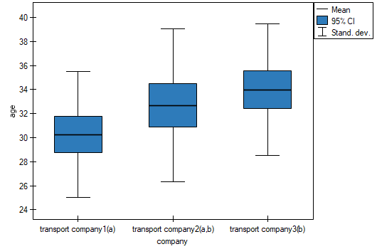
 Tukey HSD and Add graph.

The critical difference (CD) calculated for each pair of comparisons is the same (because the groups sizes are equal) and counts to 2.730855. The comparison of the  value with the value of the mean difference indicates, that there are significant differences only between the mean age of the workers from the first and the third transport company (only if these 2 groups are compared, the value is less than the difference of the means). The same conclusion you draw, if you compare the p-value of POST-HOC test with the significance level . The workers of the first transport company are about 3 years younger (on average) than the workers of the third transport company. Two interlocking homogeneous groups were obtained, which are also marked on the graph.
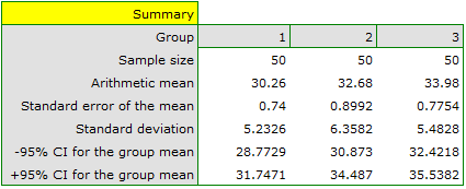
We can provide a detailed description of the data by selecting Descriptive statistics in the analysis window 
The contrasts and the POST-HOC tests
An analysis of the variance enables you to get information only if there are any significant differences among populations. It does not inform you which populations are different from each other. To gain some more detailed knowledge about the differences in particular parts of our complex structure, you should use contrasts (if you do the earlier planned and usually only particular comparisons), or the procedures of multiple comparisons POST-HOC tests (when having done the analysis of variance, we look for differences, usually between all the pairs).
The number of all the possible simple comparisons is calculated using the following formula:

Hypotheses:
The first example - simple comparisons (comparison of 2 selected means):

The second example - complex comparisons (comparison of combination of selected means):
![\begin{array}{cc}
\mathcal{H}_0: & \mu_1=\frac{\mu_2+\mu_3}{2},\\[0.1cm]
\mathcal{H}_1: & \mu_1\neq\frac{\mu_2+\mu_3}{2}.
\end{array}](/lib/exe/fetch.php?media=wiki:latex:/imgf0472a7ad15f9b99bbf5ce50cb721339.png "LaTeX")
If you want to define the selected hypothesis you should ascribe the contrast value  , to each mean. The values are selected, so that their sums of compared sides are the opposite numbers, and their values of means which are not analysed count to 0.
- The first example:
 ,
,  ,
,  .
. - The second example:
 , ,
, ,  ,
,  ,…,
,…,  .
.
How to choose the proper hypothesis:

- [ii] The p-value, designated on the basis of the proper POST-HOC test, is compared with the significance level:
For simple and complex comparisons, equal-size groups as well as unequal-size groups, when the variances are equal.
- [i] The value of critical difference is calculated by using the following formula:

where:
 - is the critical value (statistic) of the F Snedecor distribution for a given significance level and degrees of freedom, adequately: 1 and .
- [ii] The test statistic is defined by:

The test statistic has the t-student distribution with degrees of freedom.
For simple comparisons, equal-size groups as well as unequal-size groups, when the variances are equal.
- [i] The value of a critical difference is calculated by using the following formula:

where:
 - is the critical value(statistic) of the F Snedecor distribution for a given significance level and and degrees of freedom.
- [ii] The test statistic is defined by:

The test statistic has the F Snedecor distribution with and degrees of freedom.
For simple comparisons, equal-size groups as well as unequal-size groups, when the variances are equal.
- [i] The value of a critical difference is calculated by using the following formula:

where:
 - is the critical value (statistic) of the studentized range distribution for a given significance level and and
  degrees of freedom.
- [ii] The test statistic is defined by:

The test statistic has the studentized range distribution with and degrees of freedom.
Info.
The algorithm for calculating the p-value and the statistic of the studentized range distribution in PQStat is based on the Lund works (1983)1). Other applications or web pages may calculate a little bit different values than PQStat, because they may be based on less precised or more restrictive algorithms (Copenhaver and Holland (1988), Gleason (1999)).
The test examining the existence of a trend can be calculated in the same situation as ANOVA for independent variables, because it is based on the same assumptions, but it captures the alternative hypothesis differently - indicating in it the existence of a trend in the mean values for successive populations. The analysis of the trend in the arrangement of means is based on contrasts Fisher LSD. By building appropriate contrasts, you can study any type of trend such as linear, quadratic, cubic, etc. Below is a table of sample contrast values for selected trends.

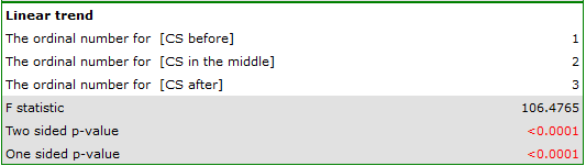
Linear trend
A linear trend, like other trends, can be analyzed by entering the appropriate contrast values. However, if the direction of the linear trend is known, simply use the For trend option and indicate the expected order of the populations by assigning them consecutive natural numbers.
The analysis is performed on the basis of linear contrast, i.e. the groups indicated according to the natural order are assigned appropriate contrast values and the statistics are calculated Fisher LSD .
With the expected direction of the trend known, the alternative hypothesis is one-sided and the one-sided  -value is interpreted. The interpretation of the two-sided -value means that the researcher does not know (does not assume) the direction of the possible trend.
The p-value, designated on the basis of the test statistic, is compared with the significance level :
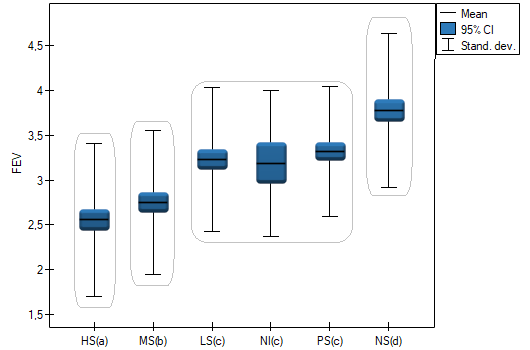
For each post-hoc test, homogeneous groups are constructed. Each homogeneous group represents a set of groups that are not statistically significantly different from each other. For example, suppose we divided subjects into six groups regarding smoking status: Nonsmokers (NS), Passive smokers (PS), Noninhaling smokers (NI), Light smokers (LS), Moderate smokers (MS), Heavy smokers (HS) and we examine the expiratory parameters for them. In our ANOVA we obtained statistically significant differences in exhalation parameters between the tested groups. In order to indicate which groups differ significantly and which do not, we perform post-hoc tests. As a result, in addition to the table with the results of each pair of comparisons and statistical significance in the form of :
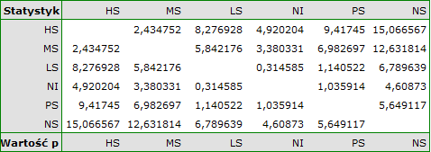
we obtain a division into homogeneous groups:
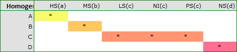
In this case we obtained 4 homogeneous groups, i.e. A, B, C and D, which indicates the possibility of conducting the study on the basis of a smaller division, i.e. instead of the six groups we studied originally, further analyses can be conducted on the basis of the four homogeneous groups determined here. The order of groups was determined on the basis of weighted averages calculated for particular homogeneous groups in such a way, that letter A was assigned to the group with the lowest weighted average, and further letters of the alphabet to groups with increasingly higher averages.
The settings window with the One-way ANOVA for independent groups can be opened in Statistics menu→Parametric tests→ANOVA for independent groups or in ''Wizard''.
The ANOVA for independent groups with F* and F" corrections
 (Brown-Forsythe, 19742)) and
  (Welch, 19513)) Corrections concern ANOVA for independent groups and are calculated when the assumption of equality of variances is not met.
The test statistic is in the form of:


where:
 – group standard deviation
  ,
,
 – group weight ,
 – weighted mean,
 .
.
This statistic is subject toSnedecor's F distribution with  and adjusted
  degrees of freedom.
The p-value, designated on the basis of the test statistic, is compared with the significance level :
POST-HOC Tests
Introduction to the contrasts and POST-HOC tests was done in chapter concerning one-way analysis of variance.
For simple and complex comparisons, equal-size groups as well as unequal-size groups, when the variances differ significantly (Tamhane A. C., 19774)).
- [i] The value of critical difference is calculated by using the following formula:

where:
 - is the critical value (statistics) of the Snedecor's F distribution for modified significance level
  and for degrees of freedom 1 and
  respectively,
 ,
,

- [ii] The test statistic is in the form of:

This statistic is subject to the t-Student distribution with  degrees of freedom, and p-value is adjusted by the number of possible simple comparisons.
BF test (Brown-Forsythe)
For simple and complex comparisons, equal-size groups as well as unequal-size groups, when the variances differ significantly (Brown M. B. i Forsythe A. B. (1974)5)).
- [i] The value of critical difference is calculated by using the following formula:

where:
 - is the critical value (statistics) of the Snedecor's F distribution for a given significance level as well as and degrees of freedom.
- [ii] The test statistic is in the form of:
 This statistic is subject to Snedecor's F distribution with and degrees of freedom.
GH test (Games-Howell).
For simple and complex comparisons, equal-size groups as well as unequal-size groups, when the variances differ significantly (Games P. A. i Howell J. F. 19766)).
- [i] The value of critical difference is calculated by using the following formula:

gdzie:
 - is the critical value (statistics) of the the distribution of the studentised interval for a given significance level as well as and degrees of freedom.
- [ii] The test statistic is in the form of:
 This statistic follows a studenty distribution with and degrees of freedom.
Trend test.
The test examining the presence of a trend can be calculated in the same situation as ANOVA for independent groups with correction and , because it is based on the same assumptions, however, differently captures the alternative hypothesis - indicating the existence of a trend in the mean values for successive populations. The analysis of the trend of the arrangement of means is based on contrasts (T2 Tamhane). By creating appropriate contrasts you can study any type of trend e.g. linear, quadratic, cubic, etc. A table of sample contrast values for certain trends can be found in the description trend test for Ona-Way ANOVA.
Linear trend
A linear trend, like other trends, can be analyzed by entering the appropriate contrast values. However, if the direction of the linear trend is known, simply use the Linear Trend option and indicate the expected order of the populations by assigning them consecutive natural numbers.
The analysis is performed based on linear contrast, i.e., the groups indicated according to the natural ordering are assigned appropriate contrast values and the T2 Tamhane statistic is calculated.
With the expected direction of the trend being known, the alternative hypothesis is one-sided and the one-sided value of is subject to interpretation. The interpretation of the two-sided value of means that the researcher does not know (does not assume) the direction of the possible trend.
The p-value, designated on the basis of the test statistic, is compared with the significance level :
Settings window for the One-way ANOVA for independent groups with F* and F„ adjustments is opened via menu Statistics→Parametric tests→ANOVA for independent groups or via the ''Wizard''.
EXAMPLE (unemployment.pqs file)
There are many factors that control the time it takes to find a job during an economic crisis. One of the most important may be the level of education. Sample data on education and time (in months) of unemployment are gathered in the file. We want to see if there are differences in average job search time for different education categories.
Hypotheses:

Due to differences in variance between populations (for Levene test  and for Brown-Forsythe test
  ):
):

the analysis is performed with the correction of various variances enabled. The obtained result of the adjusted  statistic is shown below.
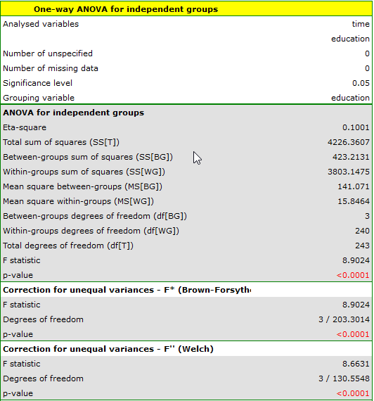
Comparing  (for the test) and (for the test) with a significance level of , we find that the average job search time differs depending on the education one has. By performing one of the POST-HOC tests, designed to compare groups with different variances, we find out which education categories are affected by the differences found:
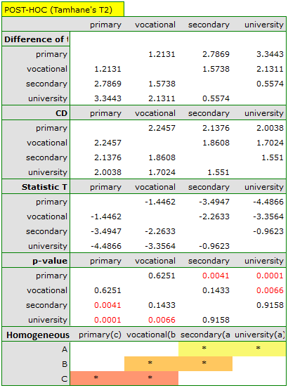
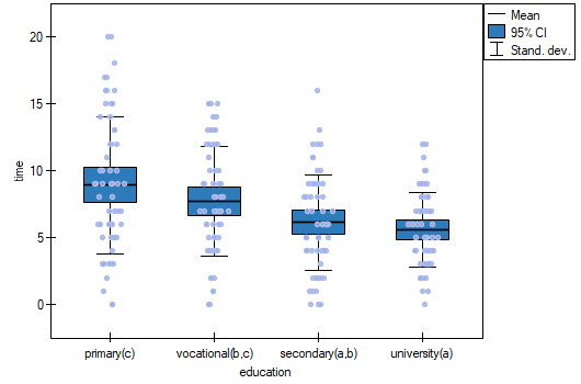
The least significant difference (LSD) determined for each pair of comparisons is not the same (even though the group sizes are equal) because the variances are not equal. Relating the LSD value to the resulting differences in mean values yields the same result as comparing the p-value with a significance level of . The differences are between primary and higher education, primary and secondary education, and vocational and higher education. The resulting homogeneous groups overlap. In general, however, looking at the graph, we might expect that the more educated a person is, the less time it takes them to find a job.
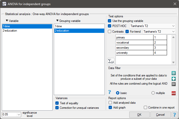
In order to test the stated hypothesis, it is necessary to perform the trend analysis. To do so, we {reopen the analysis} with the button and, in the test options window, select: the Tamhane's T2 method, the Contrasts option (and set the appropriate contrast), or the For trend option (and indicate the order of education categories by specifying consecutive natural numbers).
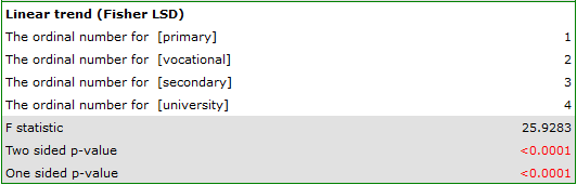
Depending on whether the direction of the correlation between education and job search time is known to us, we use a one-sided or two-sided p-value. Both of these values are less than the given significance level. The trend we predicted is confirmed, that is, at a significance level of we can say that this trend does indeed exist in the population from which the sample is drawn.
The Brown-Forsythe test and the Levene test
Both tests: the Levene test (Levene, 1960 7)) and the Brown-Forsythe test (Brown and Forsythe, 1974 8)) are used to verify the hypothesis determining the equality of variance of an analysed variable in several ( ) populations.
Basic assumptions:
- measurement on an interval scale,
- normality of distribution of an analysed feature in each population,
Hypotheses:

where:
 ,
, ,…,
,…,
 variances of an analysed variable of each population.
The analysis is based on calculating the absolute deviation of measurement results from the mean (in the Levene test) or from the median (in the Brown-Forsythe test), in each of the analysed groups. This absolute deviation is the set of data which are under the same procedure performed to the analysis of variance for independent groups. Hence, the test statistic is defined by:
The test statistic has the F Snedecor distribution with and degrees of freedom.
The p-value, designated on the basis of the test statistic, is compared with the significance level :
Note
The Brown-Forsythe test is less sensitive than the Levene test, in terms of an unfulfilled assumption relating to distribution normality.
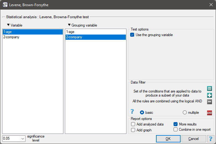
The settings window with the Levene, Brown-Forsythe tests' can be opened in Statistics menu→Parametric tests→Levene, Brown-Forsythe.
The ANOVA for dependent groups
The single-factor repeated-measures analysis of variance (ANOVA for dependent groups) is used when the measurements of an analysed variable are made several times () each time in different conditions (but we need to assume that the variances of the differences between all the pairs of measurements are pretty close to each other).
This test is used to verify the hypothesis determining the equality of means of an analysed variable in several () populations.
Basic assumptions:
- measurement on an interval scale,
- the normal distribution for all variables which are the differences of measurement pairs (or the normal distribution for an analysed variable in each measurement),
Hypotheses:
where:
,,…, – means for an analysed features, in the following measurements from the examined population.
The test statistic is defined by:

where:
 – mean square between-conditions,
 – mean square residual,
 – between-conditions sum of squares,
 – residual sum of squares,
 – total sum of squares,
 – between-subjects sum of squares,
 – between-conditions degrees of freedom,
 – residual degrees of freedom,
– total degrees of freedom,
 – between-subjects degrees of freedom,
 ,
,
 – sample size,
– values of the variable from  subjects
  in conditions .
The test statistic has the F Snedecor distribution with  and
and  degrees of freedom.
The p-value, designated on the basis of the test statistic, is compared with the significance level :
Effect size - partial <latex>$\eta^2$</latex>
This quantity indicates the proportion of explained variance to total variance associated with a factor. Thus, in a repeated measures model, it indicates what proportion of the between-conditions variability in outcomes can be attributed to repeated measurements of the variable.

Testy POST-HOC
Introduction to the contrasts and the POST-HOC tests was performed in the \ref{post_hoc} unit, which relates to the one-way analysis of variance.
For simple and complex comparisons (frequency in particular measurements is always the same).
Hypotheses:
Example - simple comparisons (comparison of 2 selected means):

- [i] The value of the critical difference is calculated by using the following formula:

where:
 - is the critical value (statistic) of the F Snedecor distribution for a given significance level and degrees of freedom, adequately: 1 and .
- [ii] The test statistic is defined by:

The test statistic has the t-Student distribution with degrees of freedom.
Note!
For contrasts  is used instead of
  , and degrees of freedem:
  .
.
For simple comparisons (frequency in particular measurements is always the same).
- [i] The value of the critical difference is calculated by using the following formula:

where:
 - is the critical value (statistic) of the F Snedecor distribution for a given significance level and and degrees of freedom.
- [
 ] The test statistic is defined by:
 The test statistic has the F Snedecor distribution with and
  degrees of freedom.
For simple comparisons (frequency in particular measurements is always the same).
- [i] The value of the critical difference is calculated by using the following formula:

where:
 - is the critical value (statistic) of the studentized range distribution for a given significance level and and degrees of freedom.
- [ii] The test statistic is defined by:

The test statistic has the studentized range distribution with and degrees of freedom.
Info.
The algorithm for calculating the p-value and statistic of the studentized range distribution in PQStat is based on the Lund works (1983)\cite{lund}. Other applications or web pages may calculate a little bit different values than PQStat, because they may be based on less precised or more restrictive algorithms (Copenhaver and Holland (1988), Gleason (1999)).
Test for trend.
The test that examines the existence of a trend can be calculated in the same situation as ANOVA for dependent variables, because it is based on the same assumptions, but it captures the alternative hypothesis differently – indicating in it the existence of a trend of mean values in successive measurements. The analysis of the trend in the arrangement of means is based on contrasts Fisher LSD test. By building appropriate contrasts, you can study any type of trend, e.g. linear, quadratic, cubic, etc. A table of example contrast values for selected trends can be found in the description of the testu dla trendu for ANOVA of independent variables.
Linear trend
Trend liniowy, tak jak pozostałe trendy, możemy analizować wpisując odpowiednie wartości kontrastów. Jeśli jednak znany jest kierunek trendu liniowego, wystarczy skorzystać z opcji Trend liniowy i wskazać oczekiwaną kolejność populacji przypisując im kolejne liczby naturalne.
A linear trend, like other trends, can be analyzed by entering the appropriate contrast values. However, if the direction of the linear trend is known, simply use the Fisher LSD test option and indicate the expected order of the populations by assigning them consecutive natural numbers.
With the expected direction of the trend known, the alternative hypothesis is one-sided and the one-sided p-values is interpreted. The interpretation of the two-sided p-value means that the researcher does not know (does not assume) the direction of the possible trend.
The p-value, designated on the basis of the test statistic, is compared with the significance level :
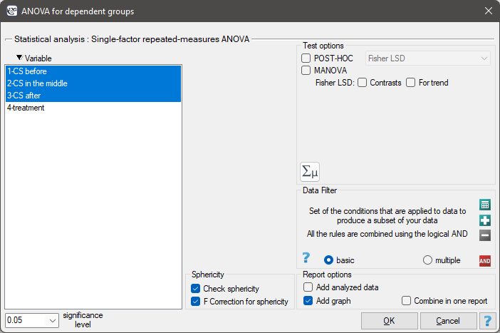
The settings window with the Single-factor repeated-measures ANOVA can be opened in Statistics menu→Parametric tests→ANOVA for dependent groups or in ''Wizard''.
EXAMPLE (pressure.pqs file)
The ANOVA for dependent groups with Epsilon correction and MANOVA
Epsilon and MANOVA corrections apply to repeated measurements ANOVA and are calculated when the assumption of sphericity is not met or the variances of the differences between all pairs of measurements are not close to each other.
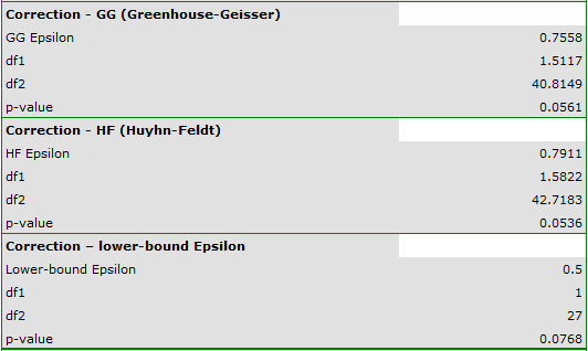
Correction of non-sphericity
The degree to which sphericity is met is represented by the value of  in the Mauchly test, but also by the values of Epsilon (
 ) calculated with corrections.
  indicates strict adherence to the sphericity condition. The smaller the value of Epsilon is compared to 1, the more the sphericity assumption is affected. The lower limit that Epsilon can reach is
  .
.
To minimize the effects of non-sphericity, three corrections can be used to change the number of degrees of freedom when testing from an F distribution. The simplest but weakest is the Epsilon lower bound correction. A slightly stronger but also conservative one is the Greenhouse-Geisser correction (1959)9). The strongest is the correction by Huynh-Feldt (1976)10). When sphericity is significantly affected, however, it is most appropriate to perform an analysis that does not require this assumption, namely MANOVA.
A multidimensional approach - MANOVA
MANOVA i.e. multivariate analysis of variance not assuming sphericity. If this assumption is not met, it is the most efficient method, so it should be chosen as a substitute for analysis of variance for repeated measurements. For a description of this method, see univariate MANOVA. Its use for repeated measures (without the independent groups factor) limits its application to data that are differences of adjacent measurements and provides testing of the same hypothesis as ANOVA for dependent variables.
Settings window for ANOVA for dependent groups with Epsilon correction and MANOVA is opened via menu Statistics→Parametric tests→ANOVA for dependent groups or via ''Wizard''.
The effectiveness of two treatments for hypertension was analyzed. A sample of 56 patients was collected and randomly assigned to two groups: group treated with drug A and group treated with drug B. Systolic blood pressure was measured three times in each group: before treatment, during treatment and after 6 months of treatment.
Hypotheses for treated with drug A:

The hypotheses for those treated with drug B read similar.
Since the data have a normal distribution, we begin our analysis by testing the assumption of sphericity. We perform the testing for each group separately using a multiple filter.
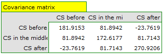
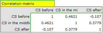
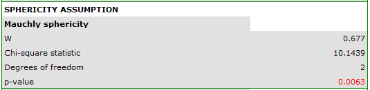
Failure to meet the sphericity assumption by the group treated with drug B is indicated by both the observed values of the covariance and correlation matrix and the result of the Mauchly test ( , p=0.0063.
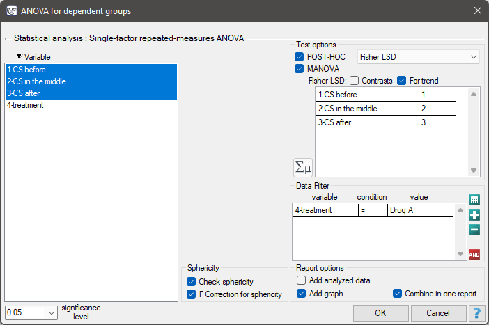
We resume our analysis and in the test options window select the primary filter to perform a repeated-measures ANOVA - for those treated with drug A, followed by a correction of this analysis and a MANOVA statistic - for those treated with drug B.
Results for those treated with drug A:
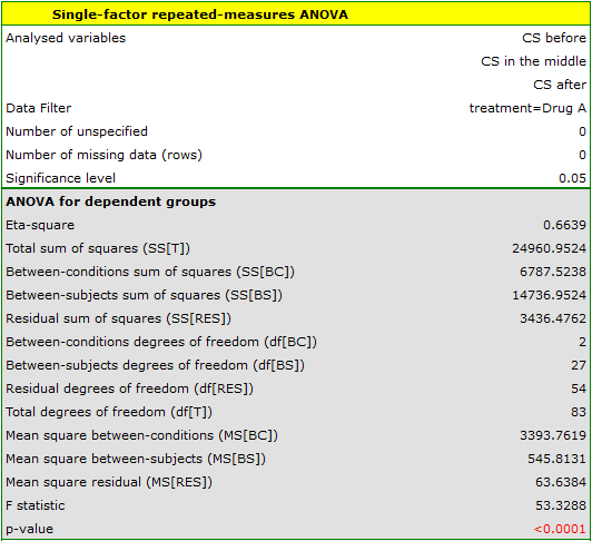
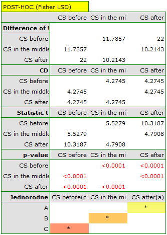
indicate significant (at the level of significance ) differences between mean systolic blood pressure values (p<0.0001 for repeated measures ANOVA). More than 66% of the between-conditions variation in outcomes can be explained by the use of drug A ( ). The differences apply to all treatment stages compared (POST-HOC score). The decrease in systolic blood pressure due to treatment is also significant (p<0.0001). Thus, we can consider Drug A as an effective drug.
Results for those treated with drug B:

indicate that there are no significant differences between mean systolic blood pressure values, both when we use epsilon and Lambda Wilks (MANOVA) corrections. As little as 17% of the between-conditions variation in results can be explained by the use of drug B ( ).
).
Mauchly's sphericity
Sphericity assumption is similar but stronger than the assumption of equality of variance. It is met if the variances for the differences between pairs of repeated measurements are the same. Usually, the simpler but more stringent compound symmetry condition is considered in place of the sphericity assumption. This can be done because meeting the compounded symmetry condition entails meeting the sphericity assumption.
Compound symmetry condition assumes, symmetry in the covariance matrix, and therefore equality of variances (elements of the main diagonal of the covariance matrix) and equality of covariances (elements off the main diagonal of the covariance matrix).
Violating the assumption of sphericity or combined symmetry unduly reduces the conservatism of the F-test (makes it easier to reject the null hypothesis).
To check the sphericity assumption, the Mauchly test is used (1940)\cite{mauchly}. Statistical significance ( ) here implies a violation of the sphericity assumption.
Basic application conditions:
- measurement on an interval scale,
- multivariate normal distribution or normality of the distribution of each variable tested,
Hypotheses:

where:
 - population variance of differences between -th pair of repeated measurements,
 - number of pairs.
Mauchly's value is defined as follows:

The test statistic has the form of:

where:
 ,
,
 - eigenvalue of the expected covariance matrix,
- number of variables analyzed.
This statistic has asymptotically (for large sample) Chi-square distribution with  degrees of freedom.
The p-value, designated on the basis of the test statistic, is compared with the significance level :
A value of  is an indication that the sphericity assumption is met. In interpreting the results of this test, however, it is important to note that it is sensitive to violations of the normality assumption of the distribution.
EXAMPLE (pressure.pqs file)
1)
Lund R.E., Lund J.R. (1983), Algorithm AS 190, Probabilities and Upper Quantiles for the Studentized Range. Applied Statistics; 34
2)
Brown M. B., Forsythe A. B. (1974), The small sample behavior of some statistics which test the equality of several means. Technometrics, 16, 385-389
3)
Welch B. L. (1951), On the comparison of several mean values: an alternative approach. Biometrika 38: 330–336
4)
Tamhane A. C. (1977), Multiple comparisons in model I One-Way ANOVA with unequal variances. Communications in Statistics, A6 (1), 15-32
5)
Brown M. B., Forsythe A. B. (1974), The ANOVA and multiple comparisons for data with heterogeneous variances. Biometrics, 30, 719-724
6)
Games P. A., Howell J. F. (1976), Pairwise multiple comparison procedures with unequal n's and/or variances: A Monte Carlo study. Journal of Educational Statistics, 1, 113-125
7)
Levene H. (1960), Robust tests for the equality of variance. In I. Olkin (Ed.) Contributions to probability and statistics (278-292). Palo Alto, CA: Stanford University Press
8)
Brown M.B., Forsythe A. B. (1974a), Robust tests for equality of variances. Journal of the American Statistical Association, 69,364-367
9)
Greenhouse S. W., Geisser S. (1959), On methods in the analysis of profile data. Psychometrika, 24, 95–112
10)
Huynh H., Feldt L. S. (1976), Estimation of the Box correction for degrees of freedom from sample data in randomized block and split=plot designs. Journal of Educational Statistics, 1, 69–82
en/statpqpl/porown3grpl/parpl.txt · ostatnio zmienione: 2022/02/12 16:23 przez admin
Narzędzia strony
Wszystkie treści w tym wiki, którym nie przyporządkowano licencji, podlegają licencji: CC Attribution-Noncommercial-Share Alike 4.0 International
