PQStat - Baza Wiedzy

One-dimensional normality tests

A variety of tests may be applicable in testing the normality of a distribution, each of which pays attention to slightly different aspects of the Gaussian distribution. It is impossible to identify a test that is good for every possible data set.

The basic condition for using tests of normality of distribution:

measurement on the interval scale.

Test hypotheses for normality of distribution:

$\begin{array}{cl} \mathcal{H}_0: & $the distribution of the characteristic under study in the population is normal,$\\ \mathcal{H}_1: & $the distribution of the examined characteristic in the population is different from the normal .$ \end{array}$

The p-value, designated on the basis of the test statistic, is compared with the significance level $\alpha$ :

$\begin{array}{ccl} $ if $ p \le \alpha & \Longrightarrow & $ reject $ \mathcal{H}_0 $ and accept $ \mathcal{H}_1, \\ $ if $ p > \alpha & \Longrightarrow & $ there is no reason to reject $ \mathcal{H}_0. \\ \end{array}$

Note

Testing for normality of distribution can be done for variables or for differences determined from two variables.

Kolmogorov-Smirnov test for normality

The test proposed by Kolmogorov (1933)¹⁾ is a relatively conservative test (it is more difficult to prove the non-normality of the distribution using it). It is based on the determination of the distance between the empirical and theoretical normal distribution. It is recommended to use it for large samples, but it should be used when the mean ( $\mu$ ) and standard deviation ( $\sigma$ ) for the population from which the sample is drawn are known. We can then check that the distribution conforms to the distribution defined by the given mean and standard deviation.

Based on the sample data collected in the cumulative frequency distribution and the corresponding values of the area under the theoretical normal distribution curve, we determine the value of the test statistic $D$ :

$\begin{displaymath} D=\sup_x{|F_n(x)-F(x)|}, \end{displaymath}$

where:

$F_n(x)$ – empirical cumulative distribution of the normal curve computed at individual points of the distribution, for $n$ -element sample ,

$F(x)$ – theoretical cumulative distribution of the normal curve.

Statystyka testu podlega rozkładowi Kołmogorova-Smirnova.

Lilliefors test for normality

A test proposed by Lilliefors (1967, 1969, 1973)²⁾, ³⁾, ⁴⁾. It is a correction of the Kolmogorov-Smirnov test when the mean ( $\mu$ ) and standard deviation ( $\sigma$ ) are unknown for the population from which the sample is drawn. It is considered slightly less conservative than the Kolmogorov-Smirnov test.

The test statistic $D$ is determined by the same formula used by the Kolmogorov-Smirnov test, but follows a Lilliefors distribution.

Shapiro-Wilk test for normality

Proposed by Shapiro and Wilk (1965)⁵⁾ for sparse groups, and adapted for more numerous groups (up to 5000 objects) by Royston (1992)⁶⁾⁷⁾. This test has a relatively high power, which makes it easier to prove the non-normality of the distribution.

The idea of how the test works is shown in the Q-Q plot.

The Shapiro-Wilk test statistic has the form:

$\begin{displaymath} W=\frac{\sum_{i=1}^na_ix_i}{\sum_{i=1}^n(x_i-\overline{x})^2}, \end{displaymath}$

where:

$a_i$ – coefficients determined based on expected values for ordered statistics, assigned weights, and covariance matrix,

$\overline{x}$ – average value of sample data.

This statistic is transformed to a statistic with a normal distribution:

$\begin{displaymath} Z=\frac{g(W)-\mu}{\sigma}, \end{displaymath}$

where:

$g(W)$ , $\mu$ i $\sigma$ – depend on the sample size:

– for small sample sizes $n\in<4;12)$ :

$g(W)=-\ln(\gamma-\ln(1-W))$ ,

$\gamma=0.459n-2.273$ ,

$\mu=-0.0006714n^3+0.025054n^2-0.39978n+0.5440$ ,

$\sigma=\exp(-0.0020322n^3+0.062767n^2-0.77857n+1.3822)$ ;

– for large sample sizes $n\in<12;5000>$ :

$g(W)=\ln(1-W)$ ,

$\mu=0.0038915u^3-0.083751u^2-0.31082u-1.5851$ ,

$\sigma=\exp(0.0030302u^2-0.082676u-0.4803)$ ,

$u=\ln(n)$ .

D'Agostino-Pearson test for normality

Different types of statistical analyses that assume normality are sensitive to different degrees to different types of departure from this assumption. Tests that refer to means in their hypotheses are assumed to be more sensitive to skewness, and tests that compare variances are assumed to depend more on kurtosis.

A normal distribution should be characterized by zero skewness and zero kurtosis g2 (or b2 close to the value three). If the distribution is not normal, as found by the D'Agostino (1973)⁸⁾ test, one can check whether this is the result of high skewness or kurtosis by the skewness test and the kurtosis test.

Like the Shapiro-Wilk test, the D'Agostino test has higher power than the Kolmogorov-Smirnov test and the Lilliefors test (D'Agostino 1990⁹⁾).

The test statistic is of the form:

$\begin{displaymath} K^2=Z_A^2+Z_K^2, \end{displaymath}$

where:

$Z_A^2$ – test statistic for the skewness,

$Z_K^2$ – test statistic for kurtosis.

This statistic has an asymptotically Chi-square distribution with two degrees of freedom.

D'Agostino skewness test

Hypotheses:

$\begin{array}{cl} \mathcal{H}_0: & $distribution is not skewed (skewness in the population is zero),$\\ \mathcal{H}_1: & $the distribution is skewed (skewness in the population deviates from zero).$ \end{array}$

The test statistic has the form:

$\begin{displaymath} Z_A=\delta\ln\left(\frac{Y}{\alpha}+\sqrt{\frac{Y^2}{\alpha^2}+1}\right), \end{displaymath}$

where:

$Y=\sqrt{(b_1)}\sqrt{\frac{(n+1)(n+3)}{6(n-2)}}$ ,

$\sqrt{(b_1)}=\frac{m_3}{m_2^{(3/2)}}$ ,

$m_k=\frac{\sum_{i=1}^{n}(x_i-\overline{x})^k}{n}$ ,

$\beta(\sqrt{(b_1)})=\frac{3(n^2+27n-70)(n+1)(n+3)}{(n-2)(n+5)(n+7)(n+9)}$ ,

$W^2=-1+\sqrt{2(\beta(\sqrt{(b_1)})-1}$ ,

$\delta=\frac{1}{\sqrt{\ln W}}$ ,

$\alpha=\sqrt{\frac{2}{W^2-1}}$ .

The statistic $Z$ has asymptotically (for large suple size) a normal distribution.

D'Agostino kurtosis test

Hypotheses:

$\begin{array}{cl} \mathcal{H}_0: & $kurtosis in the population corresponds to the kurtosis of a normal distribution,$\\ \mathcal{H}_1: & $the kurtosis in the population differs from the kurtosis of a normal distribution.$ \end{array}$

The test statistic has the form:

$\begin{displaymath} Z_K=\frac{\left(1-\frac{2}{9H}\right)-\left(\frac{1-\frac{2}{A}}{1+x\sqrt{\frac{2}{H-4}}}\right)^{1/3}}{\sqrt{\frac{2}{9H}}}, \end{displaymath}$

where:

$E(b_2)=\frac{3(n-1)}{n+1}$ ,

$b_2=\frac{m_4}{m_2^2}$ ,

$var(b_2)=\frac{24n(n-2)(n-3)}{(n+1)^2(n+3)(n+5)}$ ,

$x=\frac{b_2-E(b_2)}{\sqrt{var(b_2)}}$ ,

$\sqrt{\beta(b_2)}=\frac{6(n^2-5n+2)}{(n+7)(n+9)}\sqrt{\frac{6(n+3)(n+5)}{n(n-2)(n-5)}}$ ,

$H=6+\frac{8}{\sqrt{\beta(b_2)}}\left(\frac{2}{\sqrt{\beta(b_2)}}+\sqrt{1+\frac{4}{\beta(b_2)}}\right)$ .

The statistic $Z$ has asymptotically (for large suple size) a normal distribution.

Quantile-Quantile plot (Q-Q plot)

A quantile-quantile type plot is used to show the correspondence of two distributions. When testing the fit of a normal distribution, it checks the fit of the data distribution (empirical distribution) to a Gaussian theoretical distribution. From it, you can visually see how well the normal distribution curve fits the data. If the quantiles of the theoretical distribution and the empirical distribution match, then the points are distributed along the line $y=x$ . The horizontal axis represents the quantiles of the normal distribution, the vertical axis the quantiles of the data distribution

Various deviations from the normal distribution are possible – the interpretation of some of the most common ones is described in the diagram:

data spread out on the line, but a few points deviate strongly from the line

– there are outliers in the data
points on the left side of the graph are above the line and on the right side are below the line

– the distribution is characterized by a greater presence of outliers from the mean than is the case in a normal distribution (negative kurtosis)
points on the left side of the graph are below the line and the points on the right side are above the line

– the distribution is characterized by a smaller presence of values away from the mean than is the case in a normal distribution (positive kurtosis)
points on the left and right sides of the graph are above the line

– right-skewed distribution (positive skewness);
points on the left and right sides of the graph are below the line

– left-skewed distribution (negative skewness).

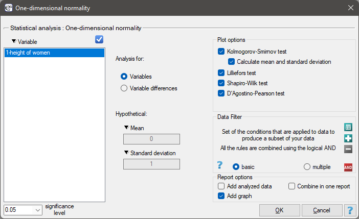
The window with the settings for the normality tests options is invoked via the Statistics→Normality tests→One-dimensional normality menu or via ''Wizard''.

EXAMPLE (Gauss.pqs file)

Women's growth

Let us assume that the height of women is such a characteristic, for which the average value is 168cm. Most of the women we meet every day are of a height not significantly different from this average. Of course there are women who are completely short and also very tall, but relatively rarely. Since very low and very high values occur rarely, and average values often, we can expect that the distribution of height is normal. To find out, 300 randomly selected women were measured.

Hypotheses:

$\begin{array}{cl} \mathcal{H}_0: & $the height distribution of women in the study population $\\ &$is normal ,$\\ \mathcal{H}_1: & $the height distribution of women in the study population $ \\ &$is not normal.$ \end{array}$

Since we do not know the mean or standard deviation for female height, but only have an assumption about these quantities, they will be determined from the sample.

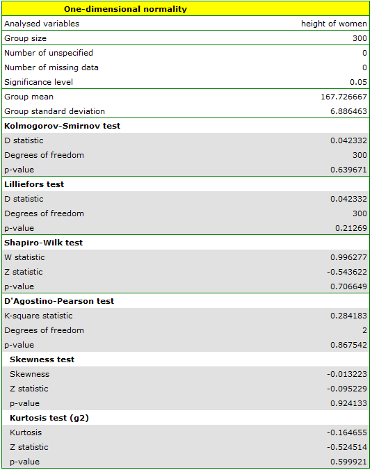
All of the designated tests indicate that there is no deviation from the normal distribution, as their $p$ values are above the standard significance level of $\alpha=0.05$ . Also, the test that examines skewness and kurtosis shows no deviation.

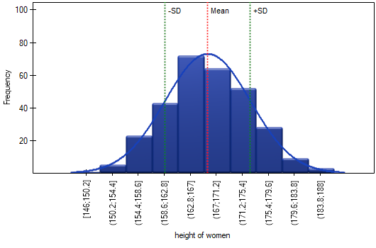
In the column chart, we presented the height distribution as 10 columns. Women between 167 cm and 171 cm are the most numerous group, while women shorter than 150 cm or taller than 184 cm are the least numerous. The bell curve of the normal distribution seems to describe this distribution well.

In the quantile-quantile plot, the points lie almost perfectly on the line, which also indicates a very good fit of the normal distribution.

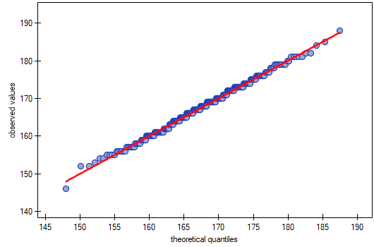
The normal distribution can therefore be regarded as the distribution that characterizes the growth of women in the population studied.

Income

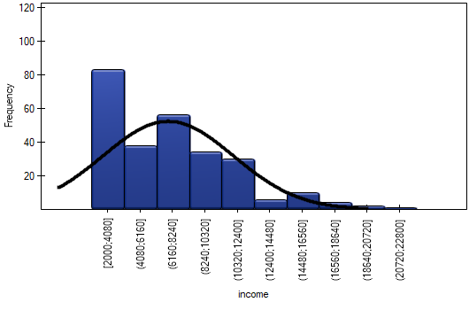
Suppose we study the income of people in a certain country. We expect that the income of most people will be average, however, there will be no people earning very little (below the minimum salary imposed by the authorities), but there will be people earning very much (company presidents), who are relatively few in number. In order to check whether the income of people in the examined country has a normal distribution, information about the income of 264 randomly selected people was collected.

Hipotezy:

$\begin{array}{cl} \mathcal{H}_0: & $the income distribution of individuals in the study population $\\ &$is a normal distribution,$\\ \mathcal{H}_1: & $the income distribution of individuals in the study population $ \\ &$is different than a normal distribution.$ \end{array}$

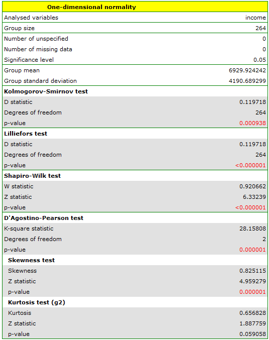
The distribution is not a normal distribution, as evidenced by all test results testing the normality of the distribution ( $p<\alpha$ ). A positive and statistically significant ( $p<\alpha$ ) skewness value indicates that the right tail of the function is too long. The function distribution is also more slender than the normal distribution, but this is not a statistically significant difference (kurtosis test).

In a quartile-quartile plot, the deviation from the normal distribution is illustrated by right-hand skewness, i.e., the location of the initial and final points of the plot significantly above the line.

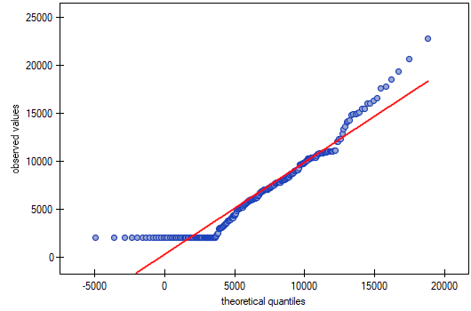
As a result, the data collected do not show that the income distribution is consistent with a normal distribution.

¹⁾

Kolmogorov A.N. (1933), Sulla deterrninazione empirica di una legge di distribuzione. Giornde1l'Inst. Ital. degli. Art., 4, 89-91

²⁾

Lilliefors H.W. (1967), On the Kolmogorov-Smimov test for normality with mean and variance unknown. Journal of the American Statistical Association, 62,399-402

³⁾

Lilliefors H.W. (1969), On the Kolmogorov-Smimov test for the exponential distribution with mean unknown. Journal of the American Statistical Association, 64,387-389

⁴⁾

Lilliefors H.W. (1973), The Kolmogorov-Smimov and other distance tests for the gamma distribution and for the extreme-value distribution when parameters must be estimated. Department of Statistics, George Washington University, unpublished manuscript

⁵⁾

Shapiro S.S. and Wilk M.B. (1965), An analysis of variance test for normality (complete samples). Biometrika 52 (3–4): 591–611

⁶⁾

Royston P. (1992), Approximating the Shapiro–Wilk W-test for non-normality„. Statistics and Computing 2 (3): 117–119

⁷⁾

Royston P. (1993b), A toolkit for testing for non-normality in complete and censored samples. Statistician 42: 37–43

⁸⁾

D'Agostino R.B. and Pearson E.S. (1973), Tests of departure from normality. Empirical results for the distribution of b2 and sqrt(b1). Biometrika, 60, 613-622

⁹⁾

D'Agostino R.B., Belanger A., D'Agostino Jr.R B. (1990), A suggestion for using powerful and informative tests of normality. American Statistician, 44, 3 16-321

PQStat - Baza Wiedzy

Narzędzia użytkownika

Narzędzia witryny

Pasek boczny

One-dimensional normality tests

Narzędzia strony