Narzędzia użytkownika
Narzędzia witryny
Pasek boczny
en:statpqpl:porown3grpl:nparpl:durbinpl
The Durbin's ANOVA (missing data)
Durbin's analysis of variance of repeated measurements for ranks was proposed by Durbin (1951)1). This test is used when measurements of the variable under study are made several times – a similar situation in which Friedman'sANOVA is used. The original Durbin test and the Friedman test give the same result when we have a complete data set. However, Durbin's test has an advantage – it can also be calculated for an incomplete data set. At the same time, data deficiencies cannot be located arbitrarily, but the data must form a so-called balanced and incomplete block:
- the number of measurements for each object is
 (
( ),
), - each measurement is made on
 objects (
 ),
), - the number of objects for which the same pair of measurements was taken simultaneously is constant and equal to
 .
.
where:
 – total number of considered measurements,
 – total number of examined objects.
Basic assumptions:
- measurement on an ordinal scale or on an interval scale,
Hypotheses involve equality of the sum of ranks for successive measurements ( ) or are simplified to medians (
 ):
):

Two test statistics of the following form are determined:
![\begin{displaymath}
T_1=\frac{(t-1)\left[\sum_{j=1}^tR_j^2-tC\right]}{A-C},
\end{displaymath}](/lib/exe/fetch.php?media=wiki:latex:/img6263bdbeddade6aabd733985ed7a7916.png "LaTeX")

where:
– sum of ranks for successive measurements  ,
,
 – ranks assigned to successive measurements, separately for each of the studied objects
  ,
,
 – sum of squared ranks,
 – correction coefficient.
The formula for  and
and  statistics includes a correction for tied ranks.
For complete data, the statistic is the same as the Friedman test. It has asymptotically (for large sample sizes) Chi-square distribution with  degrees of freedom.
The statistic is the equivalent of Friedman's Iman-Davenport ANOVA adjustment, so it follows Snedecor's F distribution with  i
i  degrees of freedom. It is now considered to be more precise than the statistic and is recommended for use with the statistic2).
The p-value, designated on the basis of the test statistic, is compared with the significance level  :
:

Testy POST-HOC
Introduction to the contrasts and the POST-HOC tests was performed in the unit, which relates to the one-way analysis of variance.
Used for simple comparisons (the counts in each measurement are always the same).
Hypotheses:
Example - simple comparisons (comparing 2 selected medians / rank sums between each other):

- [ii] The value of critical difference is calculated by using the following formula:

where:
 – is the [wartosc_krytyczna|critical value (statistic) of the t-Student distribution for a given significance level and
  degrees of freedom.
- [ii] The test statistic has the form:

The test statistic has t-Student distribution with degrees of freedom.
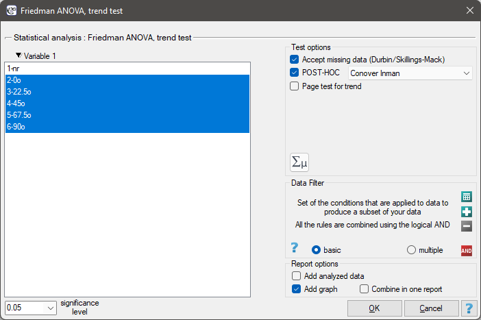
The settings window with the Durbin's ANOVA can be opened in Statistics menu→NonParametric tests →Friedman ANOVA, trend test or in ''Wizard''
Note
For records with missing data to be taken into account, you must check the Accept missing data option. Empty cells and cells with non-numeric values are treated as missing data. Only records with more than one numeric value will be analyzed.
An experiment was conducted among 20 patients in a psychiatric hospital (Ogilvie 1965)3). This experiment involved drawing straight lines according to a presented pattern. The pattern represented 5 lines drawn at different angles ( ) relative to the indicated center. The patients' task was to reproduce the lines while having their hand covered. The time at which the patient drew the line was recorded as the result of the experiment. Ideally, each patient would draw a line from all angles, but elapsed time and fatigue would have a significant impact on performance. In addition, it is difficult to keep the patient interested and willing to cooperate for an extended period of time. Therefore, the project was planned and conducted in balanced and incomplete blocks. Each of the 20 patients traced a line at two angles (there were five possible angles). Thus, each angle was drawn eight times. The time at which each patient drew a line at a given angle was recorded in the table.

We want to see if the time taken to draw each line is completely random, or if there are lines that took more or less time to draw.
Hypotheses:

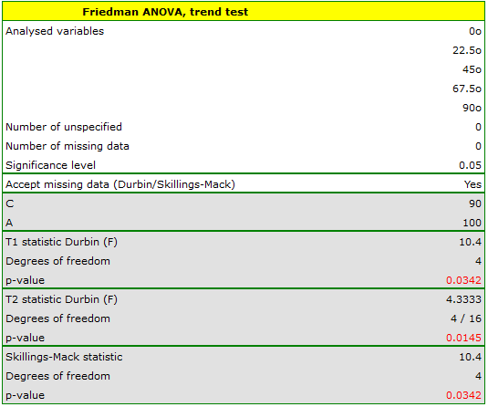
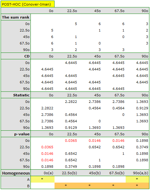
Comparing the p=0.0145 for the statistic (or the p=0.0342 for the statistic) with the  significance level, we find that the lines are not drawn at the same time. The POST-HOC analysis performed indicates that there is a difference in the time taken to draw the line at angle
  . It is drawn faster than the lines at the angle of
  ,
,  and
and  .
.
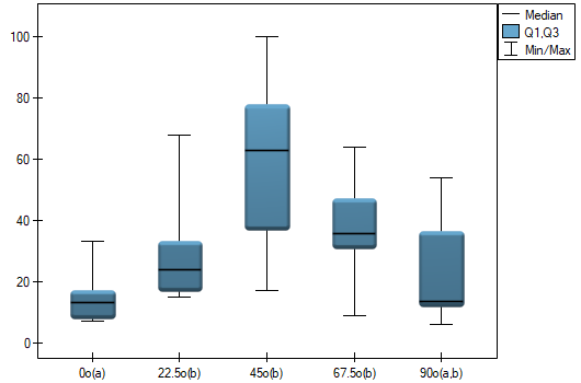
The graph shows homogeneous groups indicated by the post-hoc test.
1)
Conover W. J. (1999), Practical nonparametric statistics (3rd ed). John Wiley and Sons, New York
2)
Durbin J. (1951), Incomplete blocks in ranking experiments. British Journal of Statistical Psychology, 4: 85–90
3)
Ogilvie J. C. (1965), Paired comparison models with tests for interaction. Biometrics 21(3): 651-64
en/statpqpl/porown3grpl/nparpl/durbinpl.txt · ostatnio zmienione: 2022/02/13 17:12 przez admin
Narzędzia strony
Wszystkie treści w tym wiki, którym nie przyporządkowano licencji, podlegają licencji: CC Attribution-Noncommercial-Share Alike 4.0 International
