PQStat - Baza Wiedzy

Spis treści

Parametric tests

Parametric tests

The Fisher-Snedecor test

The F-Snedecor test is based on a variable $F$ which was formulated by Fisher (1924), and its distribution was described by Snedecor. This test is used to verify the hypothesis about equality of variances of an analysed variable for 2 populations.

Basic assumptions:

measurement on an interval scale,
normality of distribution of an analysed feature in both populations,
an independent model.

Hypotheses:

$\begin{array}{cc} \mathcal{H}_0: & \sigma_1^2=\sigma_2^2,\\ \mathcal{H}_1: & \sigma_1^2\ne\sigma_2^2, \end{array}$

where:

$\sigma_1^2$ , $\sigma_2^2$ – variances of an analysed variable of the 1st and the 2nd population.

The test statistic is defined by: $\begin{displaymath} F=\displaystyle{\frac{sd_1^2}{sd_2^2}}, \end{displaymath}$

where:

$sd_1^2$ , $sd_2^2$ – variances of an analysed variable of the samples chosen randomly from the 1st and the 2nd population.

The test statistic has the F Snedecor distribution with $n_1-1$ and $n_2-1$ degrees of freedom.

The p-value, designated on the basis of the test statistic, is compared with the significance level $\alpha$ :

$\begin{array}{ccl} $ if $ p \le \alpha & \Longrightarrow & $ reject $ \mathcal{H}_0 $ and accept $ \mathcal{H}_1, \\ $ if $ p > \alpha & \Longrightarrow & $ there is no reason to reject $ \mathcal{H}_0. \\ \end{array}$

The settings window with the Fisher-Snedecor test can be opened in Statistics menu→Parametric tests→F Fisher Snedecor.

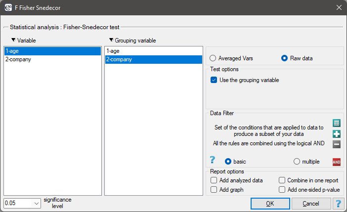
Note

Calculations can be based on raw data or data that are averaged like: arithmetic means, standard deviations and sample sizes.

2022/02/09 12:56

The t-test for independent groups

The $t$ -test for independent groups is used to verify the hypothesis about the equality of means of an analysed variable in 2 populations.

Basic assumptions:

measurement on an interval scale,
normality of distribution of an analysed feature in both populations,
an independent model,
equality of variances of an analysed variable in 2 populations.

Hypotheses:

$\begin{array}{cc} \mathcal{H}_0: & \mu_1=\mu_2,\\ \mathcal{H}_1: & \mu_1\ne\mu_2. \end{array}$

where:

$\mu_1$ , $\mu_2$ – means of an analysed variable of the 1st and the 2nd population.

The test statistic is defined by: $\begin{displaymath} t=\frac{\displaystyle{\overline{x}_1-\overline{x}_2}}{\displaystyle{\sqrt{\frac{(n_1-1)sd_1^2+(n_2-1)sd_2^2}{n_1+n_2-2}\left(\frac{1}{n_1}+\frac{1}{n_2}\right)}}}, \end{displaymath}$

where:

$\overline{x}_1, \overline{x}_2$ – means of an analysed variable of the 1st and the 2nd sample,

$n_1, n_2$ – the 1st and the 2nd sample size,

$sd_1^2, sd_2^2$ – variances of an analysed variable of the 1st and the 2nd sample.

The test statistic has the t-Student distribution with $df=n_1+n_2-2$ degrees of freedom.

The p-value, designated on the basis of the test statistic, is compared with the significance level $\alpha$ :

$\begin{array}{ccl} $ if $ p \le \alpha & \Longrightarrow & $ reject $ \mathcal{H}_0 $ and accept $ \mathcal{H}_1, \\ $ if $ p > \alpha & \Longrightarrow & $ there is no reason to reject $ \mathcal{H}_0. \\ \end{array}$

Note:

pooled standard deviation is defined by:

$\begin{displaymath} SD_p=\sqrt{\frac{(n_1-1)sd_1^2+(n_2-1)sd_2^2}{n_1+n_2-2}}, \end{displaymath}$

standard error of difference of means is defined by:

$\begin{displaymath} SE_{\overline{x}_1-\overline{x}_2}=\displaystyle{\sqrt{\frac{(n_1-1)sd_1^2+(n_2-1)sd_2^2}{n_1+n_2-2}\left(\frac{1}{n_1}+\frac{1}{n_2}\right)}}. \end{displaymath}$

Standardized effect size.

The Cohen's d determines how much of the variation occurring is the difference between the averages.

$\begin{displaymath} d=\left|\frac{\overline{x}_1-\overline{x}_2}{SD_p}\right| \end{displaymath}$ .

When interpreting an effect, researchers often use general guidelines proposed by Cohen ¹⁾ defining small (0.2), medium (0.5) and large (0.8) effect sizes.

The settings window with the t- test for independent groups can be opened in Statistics menu→Parametric tests→t-test for independent groups or in ''Wizard''.

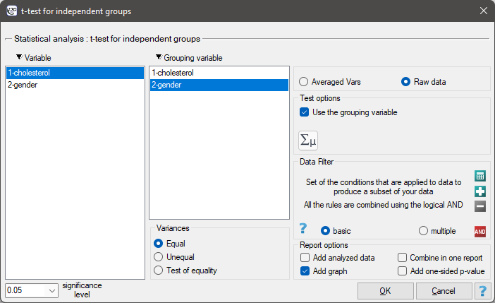
If, in the window which contains the options related to the variances, you have choosen:

equal, the t-test for independent groups will be calculated ,
different, the t-test with the Cochran-Cox adjustment will be calculated,
check equality, to calculate the Fisher-Snedecor test, basing on its result and set the level of significance, the t-test for independent groups with or without the Cochran-Cox adjustment will be calculated.

Note

Calculations can be based on raw data or data that are averaged like: arithmetic means, standard deviations and sample sizes.

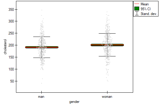
EXAMPLE (cholesterol.pqs file)

Five hundred subjects each were drawn from a population of women and a population of men over 40 years of age. The study concerned the assessment of cardiovascular disease risk. Among the parameters studied is the value of total cholesterol. The purpose of this study will be to compare men and women as to this value. We want to show that these populations differ on the level of total cholesterol and not only on the level of cholesterol broken down into its fractions.

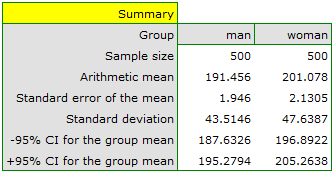
The distribution of age in both groups is a normal distribution (this was checked with the Lilliefors test). The mean cholesterol value in the male group was $\overline{x}_1=201.1$ and the standard deviation $sd_1=47.6$ , in the female group $\overline{x}_2=191.5$ and $sd_2=43.5$ respectively. The Fisher-Snedecor test indicates small but statistically significant ( $p=0.0434$ ) differences in variances. The analysis will use the Student's t-test with Cochran-Cox correction

Hypotheses:

$\begin{array}{cl} \mathcal{H}_0: & $The average total cholesterol of the female population is different from$\\ &$the average total cholesterol of the male population,$\\ \mathcal{H}_1: & $The average total cholesterol of the female population equals$ \\ &$the average total cholesterol of the male population.$ \end{array}$

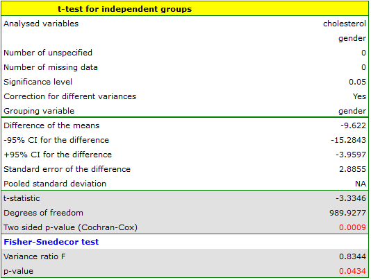
Comparing $p=0.0009$ with a significance level $\alpha=0.05$ we find that women and men in Poland have statistically significant differences in total cholesterol values. The average Polish man over the age of 40 has higher total cholesterol than the average Polish woman by almost 10 units.

2022/02/09 12:56

The t-test with the Cochran-Cox adjustment

The Cochran-Cox adjustment relates to the t-test for independent groups (1957)²⁾ and is calculated when variances of analysed variables in both populations are different.

The test statistic is defined by:

$\begin{displaymath} t=\frac{\overline{x}_1-\overline{x}_2}{\sqrt{\frac{sd_1^2}{n_1}+\frac{sd_2^2}{n_2}}}. \end{displaymath}$

The test statistic has the t-Student distribution with degrees of freedom proposed by Satterthwaite (1946)³⁾ and calculated using the formula:

$\begin{displaymath} df=\frac{\left( \frac{sd_1^2}{n_1}+\frac{sd_2^2}{n_2}\right)^2}{\left( \frac{sd_1^2}{n_1}\right)^2\cdot \frac{1}{(n_1-1)}+\left( \frac{sd_2^2}{n_2}\right)^2\cdot \frac{1}{(n_2-1)}}. \end{displaymath}$

The settings window with the t- test for independent groups can be opened in Statistics menu→Parametric tests→t-test for independent groups or in ''Wizard''.

If, in the window which contains the options related to the variances, you have choosen:

equal, the t-test for independent groups will be calculated ,
different, the t-test with the Cochran-Cox adjustment will be calculated,
check equality, to calculate the Fisher-Snedecor test, basing on its result and set the level of significance, the t-test for independent groups with or without the Cochran-Cox adjustment will be calculated.

Note Calculations can be based on raw data or data that are averaged like: arithmetic means, standard deviations and sample sizes.

2022/02/09 12:56

The t-test for dependent groups

The $t$ -test for dependent groups is used when the measurement of an analysed variable you do twice, each time in different conditions (but you should assume, that variances of the variable in both measurements are pretty close to each other). We want to check how big is the difference between the pairs of measurements ( $d_i=x_{1i}-x_{2i}$ ). This difference is used to verify the hypothesis informing us that the mean of the difference in the analysed population is 0.

Basic assumptions:

measurement on an interval scale,
normality of distribution of measurements $d_i$ (or the normal distribution for an analysed variable in each measurement),
a dependent model.

Hypotheses:

$\begin{array}{cc} \mathcal{H}_0: & \mu_0=0,\\ \mathcal{H}_1: & \mu_0\ne0, \end{array}$

where:

$\mu_0$ , – mean of the differences $d_i$ in a population.

The test statistic is defined by:

$\begin{displaymath} t=\frac{\overline{d}}{sd_d}\sqrt{n}, \end{displaymath}$

where:

$\overline{d}$ – mean of differences $d_i$ in a sample,

$sd_d$ – standard deviation of differences $d_i$ in a sample,

$n$ – number of differences $d_i$ in a sample.

Test statistic has the t-Student distribution with $n-1$ degrees of freedom.

The p-value, designated on the basis of the test statistic, is compared with the significance level $\alpha$ :

$\begin{array}{ccl} $ if $ p \le \alpha & \Longrightarrow & $ reject $ \mathcal{H}_0 $ and accept $ \mathcal{H}_1, \\ $ if $ p > \alpha & \Longrightarrow & $ there is no reason to reject $ \mathcal{H}_0. \\ \end{array}$

Note

standard deviation of the difference is defined by:

$\begin{displaymath} sd_d=\displaystyle{\sqrt{\frac{\sum_{i=1}^{n}(d_i-\overline{d})^2}{n-1}}}, \end{displaymath}$

standard error of the mean of differences is defined by:

$\begin{displaymath} SEM_{d}=\displaystyle{\frac{SD_d}{\sqrt{n}}}. \end{displaymath}$

Standardized effect size.

The Cohen's d determines how much of the variation occurring is the difference between the averages, while taking into account the correlation of the variables.

$\begin{displaymath} d=\frac{dz}{\sqrt{1-r_p}}, \end{displaymath}$ .

where:

$dz=\left|\frac{\overline{d}}{sd_d}\right|$ ,

$r_p$ – the Pearson product-moment correlation coefficient.

When interpreting an effect, researchers often use general guidelines proposed by Cohen ⁴⁾ defining small (0.2), medium (0.5) and large (0.8) effect sizes.

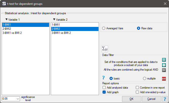
The settings window with the t-test for dependent groups can be opened in Statistics menu→Parametric tests→t-test for dependent groups or in ''Wizard''.

Note

Calculations can be based on raw data or data that are averaged like: arithmetic mean of difference, standard deviation of difference and sample size.

EXAMPLE(BMI.pqs file)

A clinic treating eating disorders studied the effect of a recommended „diet A” on weight change. A sample of 120 obese patients were put on the diet. Their BMI levels were measured twice: before the diet and after 180 days of the diet. To test the effectiveness of the diet, the obtained BMI measurements were compared.

Hypotheses:

$\begin{array}{cl} \mathcal{H}_0: & $Mean BMI values do not change with diet,$\\ \mathcal{H}_1: & $Mean BMI values change as a result of diet.$ \end{array}$

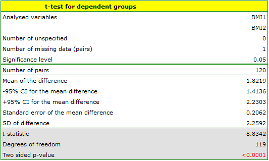
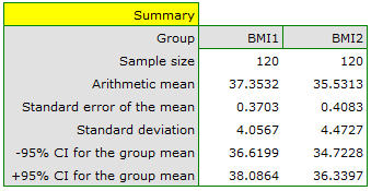
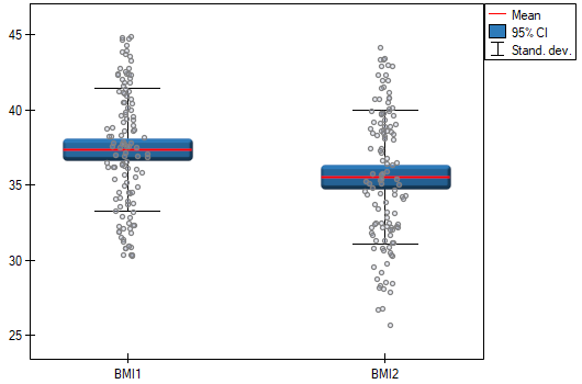
Comparing $p<0.0001$ with a significance level $\alpha=0.05$ we find that the mean BMI level changed significantly. Before the diet, it was higher by less than 2 units on average.

The study was able to use the Student's t-test for dependent groups because the distribution of the difference between pairs of measurements was a normal distribution (Lilliefors test, $p=0.0837$ ).

2022/02/09 12:56

¹⁾ , ⁴⁾

Cohen J. (1988), Statistical Power Analysis for the Behavioral Sciences, Lawrence Erlbaum Associates, Hillsdale, New Jersey

²⁾

Cochran W.G. and Cox G.M. (1957), Experimental designs (2nd 4.). New York: John Wiley and Sons.

³⁾

Satterthwaite F.E. (1946), An approximate distribution of estimates of variance components. Biometrics Bulletin, 2, 1 10-1 14

PQStat - Baza Wiedzy

Narzędzia użytkownika

Narzędzia witryny

Pasek boczny

Spis treści

Parametric tests

The Fisher-Snedecor test

The t-test for independent groups

The t-test with the Cochran-Cox adjustment

The t-test for dependent groups

Narzędzia strony