PQStat - Baza Wiedzy

The Mann-Whitney U test

The Mann-Whitney $U$ test is also called as the Wilcoxon Mann-Whitney test (Mann and Whitney (1947)¹⁾ and Wilcoxon (1949)²⁾). This test is used to verify the hypothesis that there is no shift in the compared distributions, i.e., most often the insignificance of differences between medians of an analysed variable in 2 populations (but you should assume that the distributions of a variable are pretty similar to each other - comparison of rank variances can be performed with the Conover rank test.

Basic assumptions:

measurement on an ordinal scale or on an interval scale,
an independent model.

Hypotheses:

$\begin{array}{cl} \mathcal{H}_0: & \phi_1=\phi_2,\\ \mathcal{H}_1: & \phi_1\neq\phi_2, \end{array}$

where:

$\phi_1, \phi_2$ distributions of an analysed variable of the 1st and the 2nd population.

The p-value, designated on the basis of the test statistic, is compared with the significance level $\alpha$ :

$\begin{array}{ccl} $ if $ p \le \alpha & \Longrightarrow & $ reject $ \mathcal{H}_0 $ and accept $ \mathcal{H}_1, \\ $ if $ p > \alpha & \Longrightarrow & $ there is no reason to reject $ \mathcal{H}_0. \\ \end{array}$

Note

Depending on a sample size, the test statistic is calculated using by different formulas:

For a small sample size:

$\begin{displaymath} U=n_1n_2+\frac{n_1(n_1+1)}{2}-R_1, \end{displaymath}$

or

$\begin{displaymath} U'=n_1n_2+\frac{n_2(n_2+1)}{2}-R_2, \end{displaymath}$

where $n_1, n_2$ are sample sizes, $R_1, R_2$ are rank sums for the samples.

This statistic has the Mann-Whitney distribution and it does not contain any correction for ties. The value of the exact probability of the Mann-Whitney distribution is calculated with the accuracy up to the hundredth place of the fraction.

For a large sample size:

$\begin{displaymath} Z=\frac{U-\frac{n_1n_2}{2}}{\sqrt{\frac{n_1n_2(n1+n_2+1)}{12}-\frac{n_1n_2\sum (t^3-t)}{12(n_1+n_2)(n_1+n_2-1)}}}, \end{displaymath}$

where:

$U$ can be replaced with $U'$ ,

$t$ – number of cases included in a tie.

The formula for the $Z$ statistic includes the correction for ties. This correction is used, when ties occur (if there are no ties, the correction is not calculated, because of $\frac{n_1n_2\sum (t^3-t)}{12(n_1+n_2)(n_1+n_2-1)}=0$ )

The $Z$ statistic asymptotically (for large sample sizes) has the normal distribution.

The Mann-Whitney test with the continuity correction (Marascuilo and McSweeney (1977)³⁾)

The continuity correction should be used to guarantee the possibility of taking in all the values of real numbers by the test statistic, according to the assumption of the normal distribution. The formula for the test statistic with the continuity correction is defined as:

$\begin{displaymath} Z=\frac{\left|U-\frac{n_1n_2}{2}\right|-0.5}{\sqrt{\frac{n_1n_2(n1+n_2+1)}{12}-\frac{n_1n_2\sum (t^3-t)}{12(n_1+n_2)(n_1+n_2-1)}}}. \end{displaymath}$

Standardized effect size

The distribution of the Mann-Whitney test statistic is approximated by the normal distribution, which can be converted to an effect size $r=\left|Z/(n_1+n_2)\right|$ ⁴⁾ to then obtain the Cohen's d value according to the standard conversion used for meta-analyses:

$\begin{displaymath} d=\frac{2r}{\sqrt{1-r^2}} \end{displaymath}$

When interpreting an effect, researchers often use general guidelines proposed by ⁵⁾ defining small (0.2), medium (0.5) and large (0.8) effect sizes.

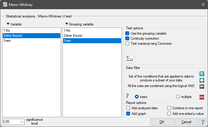
The settings window with the Mann-Whitney U test can be opened in Statistics menu → NonParametric tests (ordered categories) → Mann-Whitney or in ''Wizard''.

EXAMPLE (computer.pqs file)

There was made a hypothesis that at some university male math students spend statistically more time in front of a computer screen than the female math students. To verify the hypothesis from the population of people who study math at this university, there was drawn a sample consisting of 54 people (25 women and 29 men). These persons were asked how many hours they spend in front of the computer screens daily. There were obtained the following results:

(time, sex): (2, k) (2, m) (2, m) (3, k) (3, k) (3, k) (3, k) (3, m) (3, m) (4, k) (4, k) (4, k) (4, k) (4, m) (4, m) (5, k) (5, k) (5, k) (5, k) (5, k) (5, k) (5, k) (5, k) (5, k) (5, m) (5, m) (5, m) (5, m) (6, k) (6, k) (6, k) (6, k) (6, k) (6, m) (6, m) (6, m) (6, m) (6, m) (6, m) (6, m) (6, m) (7, k) (7, m) (7, m) (7, m) (7, m) (7, m) (7, m) (7, m) (7, m) (7, m) (8, k) (8, m) (8, m).}

Hypotheses:

$\begin{array}{cl} \mathcal{H}_0: & $the median of the time spent in front of a computer screen is exactly the same both$\\ & $in the male and the female population of students, at the analysed university,$\\ \mathcal{H}_1: & $the median of the time spent in front of a computer screen is different among the $\\ & $male population and the female population of students, at the analysed university.$ \end{array}$

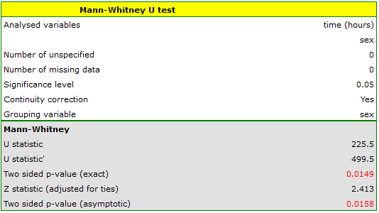
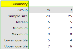
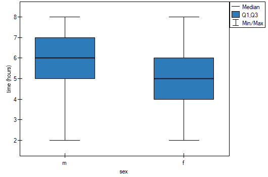
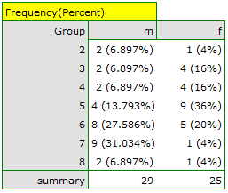
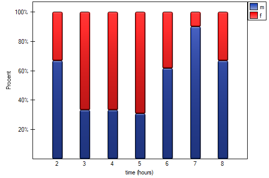
Based on the assumed $\alpha=0.05$ and the $Z$ statistic of the Mann-Whitney test without correction for continuity (p=0.0154) as well as with this correction p=0.0158, as well as on the exact $U$ statistic (p=0.0149) we can assume that there are statistically significant differences between female and male math students in the amount of time spent in front of the computer. These differences are that female students spend less time in front of the computer than male students. They can be described by the median, quartiles, and the largest and smallest value, which we also see in a box-and-whisker plot. Another way to describe the differences is to represent the time spent in front of the computer based on a table of counts and percentages (which we run in the analysis window by setting descriptive statistics includegraphics ) or based on a column plot.

¹⁾

Mann H. and Whitney D. (1947), On a test of whether one of two random variables is stochastically larger than the other. Annals of Mathematical Statistics, 1 8 , 5 0 4

²⁾

Wilcoxon F. (1949), Some rapid approximate statistical procedures. Stamford, CT: Stamford Research Laboratories, American Cyanamid Corporation

³⁾

Marascuilo L.A. and McSweeney M. (1977), Nonparametric and distribution-free method for the social sciences. Monterey, CA: Brooks/Cole Publishing Company

⁴⁾

Fritz C.O., Morris P.E., Richler J.J.(2012), Effect size estimates: Current use, calculations, and interpretation. Journal of Experimental Psychology: General., 141(1):2–18.

⁵⁾

Cohen J. (1988), Statistical Power Analysis for the Behavioral Sciences, Lawrence Erlbaum Associates, Hillsdale, New Jersey

PQStat - Baza Wiedzy

Narzędzia użytkownika

Narzędzia witryny

Pasek boczny

The Mann-Whitney U test

Narzędzia strony