PQStat - Baza Wiedzy

The Chi-square goodness-of-fit test

The $\chi^2$ test (goodnes-of-fit) is also called the one sample $\chi^2$ test and is used to test the compatibility of values observed for $r$ ( $r>=2$ ) categories $X_1, X_2,..., X_r$ of one feature $X$ with hypothetical expected values for this feature. The values of all $n$ measurements should be gathered in a form of a table consisted of $r$ rows (categories: $X_1, X_2, ..., X_r$ ). For each category $X_i$ there is written the frequency of its occurence $O_i$ , and its expected frequency $E_i$ or the probability of its occurence $p_i$ . The expected frequency is designated as a product of $E_i=np_i$ . The built table can take one of the following forms:

$\begin{tabular}[t]{c@{\hspace{1cm}}c} \begin{tabular}{c|c c} $X_i$ categories& $O_i$ & $E_i$ \\\hline $X_1$ & $O_1$ & $E_i$ \\ $X_2$ & $O_2$ & $E_2$ \\ ... & ... & ...\\ $X_r$ & $O_r$ & $E_r$ \\ \end{tabular} & \begin{tabular}{c|c c} $X_i$ categories& $O_i$ & $p_i$ \\\hline $X_1$ & $O_1$ & $p_1$ \\ $X_2$ & $O_2$ & $p_2$ \\ ... & ... & ...\\ $X_r$ & $O_r$ & $p_r$ \\ \end{tabular} \end{tabular}$

Basic assumptions:

measurement on a nominal scale - any order is not taken into account,
large expected frequencies (according to the Cochran interpretation (1952)¹⁾,
observed frequencies total should be exactly the same as an expected frequencies total, and the total of all $p_i$ probabilities should come to 1.

Hypotheses:

$\begin{array}{cl} \mathcal{H}_0: & O_i=E_i $ for all categories,$\\ \mathcal{H}_1: & O_i \neq E_i $ for at least one category.$ \end{array}$

Test statistic is defined by:

$\begin{displaymath} \chi^2=\sum_{i=1}^r\frac{(O_i-E_i)^2}{E_i}. \end{displaymath}$

This statistic asymptotically (for large expected frequencies) has the Chi-square distribution with the number of degrees of freedom calculated using the formula: $df=(r-1)$ .
The p-value, designated on the basis of the test statistic, is compared with the significance level $\alpha$ :

$\begin{array}{ccl} $ if $ p \le \alpha & \Longrightarrow & $ reject $ \mathcal{H}_0 $ and accept $ \mathcal{H}_1, \\ $ if $ p > \alpha & \Longrightarrow & $ there is no reason to reject $ \mathcal{H}_0. \\ \end{array}$

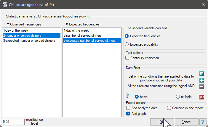
The settings window with the Chi-square test (goodness-of-fit) can be opened in Statistics menu → NonParametric tests (unordered categories)→Chi-square (goodnes-of-fit) or in ''Wizard''.

EXAMPLE (dinners.pqs file )

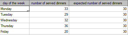
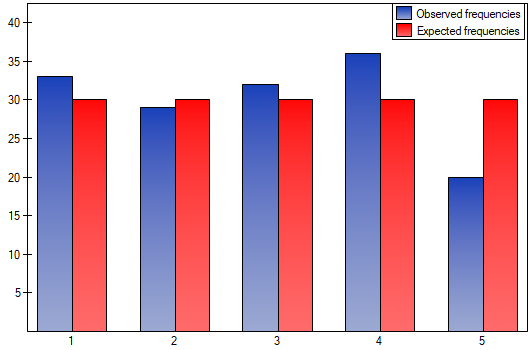
We would like to get to know if the number of dinners served in some school canteen within a given frame of time (from Monday to Friday) is statistically the same. To do this, there was taken a one-week-sample and written the number of served dinners in the particular days: Monday - 33, Tuesday - 29, Wednesday - 32, Thursday -36, Friday - 20.

As a result there were 150 dinners served in this canteen within a week (5 days). We assume that the probability of serving dinner each day is exactly the same, so it comes to $\frac{1}{5}$ . The expected frequencies of served dinners for each day of the week (out of 5) comes to $E_i=150\cdot\frac{1}{5}=30$ .

Hypotheses:

$\begin{array}{cl} \mathcal{H}_0: & $the number of served dinners in the analysed school canteen within given$\\ & $days (of the week) is consistent with the expected number of given out dinners these$\\ & $days,$\\ \mathcal{H}_1: & $the number of served out dinners in the analysed school canteen within a given $\\ & $week is not consistent with the expected number of dinners given out these days.$ \end{array}$

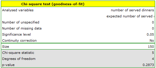
The p-value from the $\chi^2$ distribution with 4 degrees of freedom comes to 0.2873. So using the significance level $\alpha=0.05$ you can estimate that there is no reason to reject the null hypothesis that informs about the compatibility of the number of served dinners with the expected number of dinners served within the particular days.

Note!

If you want to make more comparisons within the framework of a one research, it is possible to use the Bonferroni correction²⁾. The correction is used to limit the size of I type error, if we compare the observed frequencies and the expected ones between particular days, for example:

Friday $\Longleftrightarrow$ Monday,

Friday $\Longleftrightarrow$ Tuesday,

Friday $\Longleftrightarrow$ Wednesday,

Friday $\Longleftrightarrow$ Thursday,

Provided that, the comparisons are made independently. The significance level $\alpha=0.05$ for each comparison must be calculated according to this correction using the following formula: $\alpha=\frac{0.05}{r}$ , where $r$ is the number of executed comparisons. The significance level for each comparison according to the Bonferroni correction (in this example) is $\alpha=\frac{0.05}{4}=0.0125$ .

However, it is necessary to remember that if you reduce $\alpha$ for each comparison, the power of the test is increased.

¹⁾

Cochran W.G. (1952), The chi-square goodness-of-fit test. Annals of Mathematical Statistics, 23, 315-345

²⁾

Abdi H. (2007), Bonferroni and Sidak corrections for multiple comparisons, in N.J. Salkind (ed.): Encyclopedia of Measurement and Statistics. Thousand Oaks, CA: Sage

PQStat - Baza Wiedzy

Narzędzia użytkownika

Narzędzia witryny

Pasek boczny

The Chi-square goodness-of-fit test

Narzędzia strony