PQStat - Baza Wiedzy

Spis treści

Non-parametric tests

Non-parametric tests

The Wilcoxon test (signed-ranks)

The Wilcoxon signed-ranks test is also known as the Wilcoxon single sample test, Wilcoxon (1945, 1949)¹⁾. This test is used to verify the hypothesis, that the analysed sample comes from the population, where median ( $\theta$ ) is a given value.

Basic assumptions:

measurement on an ordinal scale or on an interval scale.

Hypotheses:

$\begin{array}{cl} \mathcal{H}_0: & \theta=\theta_0, \\ \mathcal{H}_1: & \theta\neq \theta_0. \end{array}$

where:

$\theta$ – median of an analysed feature of the population represented by the sample,

$\theta_0$ – a given value.

Now you should calculate the value of the test statistics $Z$ ( $T$ – for the small sample size), and based on this $p$ value.

The p-value, designated on the basis of the test statistic, is compared with the significance level $\alpha$ :

$\begin{array}{ccl} $ if $ p \le \alpha & \Longrightarrow & $ reject $ \mathcal{H}_0 $ and accept $ \mathcal{H}_1, \\ $ if $ p > \alpha & \Longrightarrow & $ there is no reason to reject $ \mathcal{H}_0. \\ \end{array}$

Note

Depending on the size of the sample, the test statistic takes a different form:

for a small sample size

$\begin{displaymath} T=\min\left(\sum R_-,\sum R_+\right), \end{displaymath}$

where:

$\sum R_+$ and $\sum R_-$ are adequately: a sum of positive and negative ranks.

This statistic has the Wilcoxon distribution.

for a large sample size

$\begin{displaymath} Z=\frac{T-\frac{n(n+1)}{4}}{\sqrt{\frac{n(n+1)(2n+1)}{24}-\frac{\sum t^3-\sum t}{48}}}, \end{displaymath}$

where:

$n$ - the number of ranked signs (the number of ranks),

$t$ - the number of cases being included in the interlinked rank.

The test statistic formula $Z$ includes the correction for ties. This correction should be used when ties occur (when there are no ties, the correction is not calculated, because $\left(\sum t^3-\sum t\right)/48=0$ .

$Z$ statistic asymptotically (for a large sample size) has the normal distribution. Continuity correction of the Wilcoxon test (Marascuilo and McSweeney (1977)²⁾)

A continuity correction is used to enable the test statistic to take in all values of real numbers, according to the assumption of the normal distribution. Test statistic with a continuity correction is defined by:

$\begin{displaymath} Z=\frac{\left|T-\frac{n(n+1)}{4}\right|-0.5}{\sqrt{\frac{n(n+1)(2n+1)}{24}-\frac{\sum t^3-\sum t}{48}}}. \end{displaymath}$

Standardized effect size

The distribution of the Wilcoxon test statistic is approximated by the normal distribution, which can be converted to an effect size $r=\left|Z/n\right|$ ³⁾ to then obtain the Cohen's d value according to the standard conversion used for meta-analyses:

$\begin{displaymath} d=\frac{2r}{\sqrt{1-r^2}} \end{displaymath}$

When interpreting an effect, researchers often use general guidelines proposed by ⁴⁾ defining small (0.2), medium (0.5) and large (0.8) effect sizes.

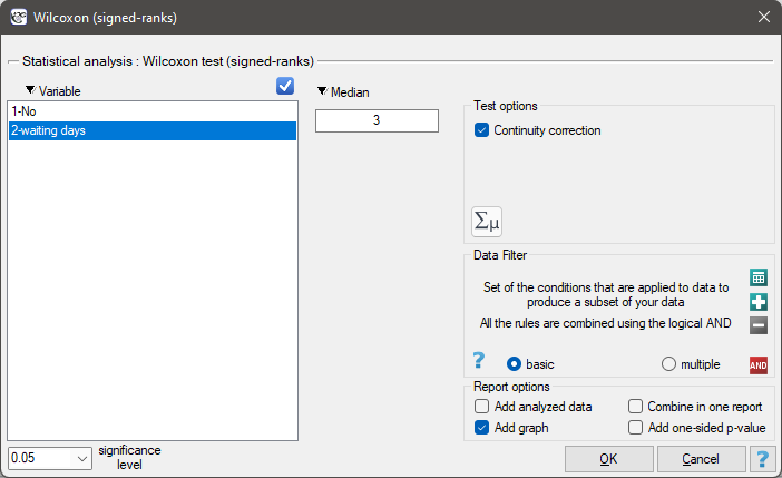
The settings window with the Wilcoxon test (signed-ranks) can be opened in Statistics menu $\to$ NonParametric tests→Wilcoxon (signed-ranks) or in ''Wizard''.

EXAMPLE cont. (courier.pqs file)

Hypotheses:

$\begin{array}{cl} \mathcal{H}_0: & $median of the number of awaiting days for the delivery, which is supposed $\\ &$to be delivered by the analysed courier company is 3$\\ \mathcal{H}_1: & $median of the number of awaiting days for the delivery, which is supposed $ \\ &$to be delivered by the analysed courier company is different from 3$ \end{array}$

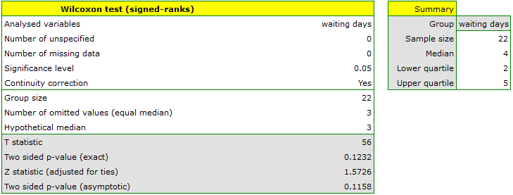
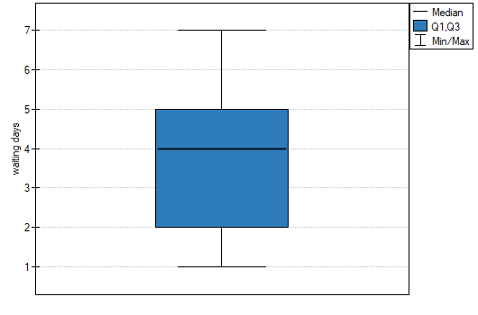
Comparing the p-value = 0.1232 of Wilcoxon test based on $T$ statistic with the significance level $\alpha=0.05$ we draw the conclusion, that there is no reason to reject the null hypothesis informing us, that usually the number of awaiting days for the delivery which is supposed to be delivered by the analysed courier company is 3. Exactly the same decision you would make basing on the p-value = 0.1112 or p-value = 0.1158 of Wilcoxon test based upon $Z$ statistic or $Z$ with correction for continuity.

2022/02/09 12:56

The Chi-square goodness-of-fit test

The $\chi^2$ test (goodnes-of-fit) is also called the one sample $\chi^2$ test and is used to test the compatibility of values observed for $r$ ( $r>=2$ ) categories $X_1, X_2,..., X_r$ of one feature $X$ with hypothetical expected values for this feature. The values of all $n$ measurements should be gathered in a form of a table consisted of $r$ rows (categories: $X_1, X_2, ..., X_r$ ). For each category $X_i$ there is written the frequency of its occurence $O_i$ , and its expected frequency $E_i$ or the probability of its occurence $p_i$ . The expected frequency is designated as a product of $E_i=np_i$ . The built table can take one of the following forms:

$\begin{tabular}[t]{c@{\hspace{1cm}}c} \begin{tabular}{c|c c} $X_i$ categories& $O_i$ & $E_i$ \\\hline $X_1$ & $O_1$ & $E_i$ \\ $X_2$ & $O_2$ & $E_2$ \\ ... & ... & ...\\ $X_r$ & $O_r$ & $E_r$ \\ \end{tabular} & \begin{tabular}{c|c c} $X_i$ categories& $O_i$ & $p_i$ \\\hline $X_1$ & $O_1$ & $p_1$ \\ $X_2$ & $O_2$ & $p_2$ \\ ... & ... & ...\\ $X_r$ & $O_r$ & $p_r$ \\ \end{tabular} \end{tabular}$

Basic assumptions:

measurement on a nominal scale - any order is not taken into account,
large expected frequencies (according to the Cochran interpretation (1952)⁵⁾,
observed frequencies total should be exactly the same as an expected frequencies total, and the total of all $p_i$ probabilities should come to 1.

Hypotheses:

$\begin{array}{cl} \mathcal{H}_0: & O_i=E_i $ for all categories,$\\ \mathcal{H}_1: & O_i \neq E_i $ for at least one category.$ \end{array}$

Test statistic is defined by:

$\begin{displaymath} \chi^2=\sum_{i=1}^r\frac{(O_i-E_i)^2}{E_i}. \end{displaymath}$

This statistic asymptotically (for large expected frequencies) has the Chi-square distribution with the number of degrees of freedom calculated using the formula: $df=(r-1)$ .
The p-value, designated on the basis of the test statistic, is compared with the significance level $\alpha$ :

$\begin{array}{ccl} $ if $ p \le \alpha & \Longrightarrow & $ reject $ \mathcal{H}_0 $ and accept $ \mathcal{H}_1, \\ $ if $ p > \alpha & \Longrightarrow & $ there is no reason to reject $ \mathcal{H}_0. \\ \end{array}$

The settings window with the Chi-square test (goodness-of-fit) can be opened in Statistics menu → NonParametric tests (unordered categories)→Chi-square (goodnes-of-fit) or in ''Wizard''.

EXAMPLE (dinners.pqs file )

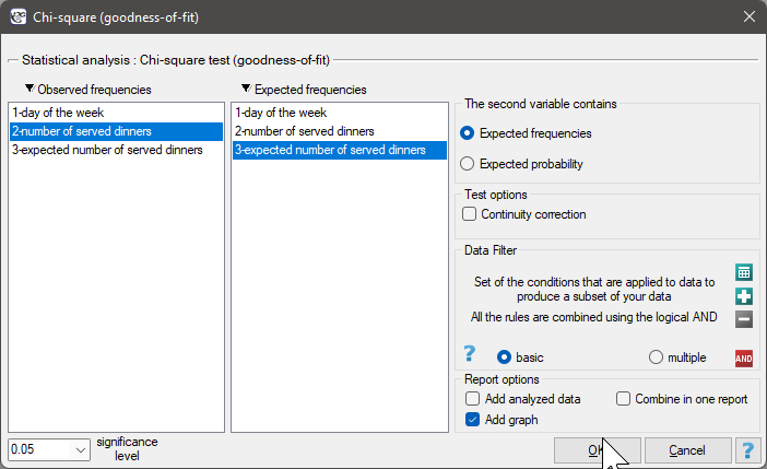
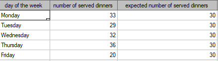
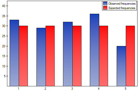
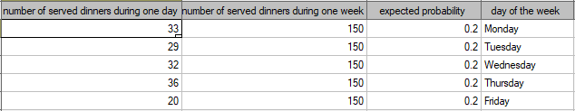
We would like to get to know if the number of dinners served in some school canteen within a given frame of time (from Monday to Friday) is statistically the same. To do this, there was taken a one-week-sample and written the number of served dinners in the particular days: Monday - 33, Tuesday - 29, Wednesday - 32, Thursday -36, Friday - 20.

As a result there were 150 dinners served in this canteen within a week (5 days). We assume that the probability of serving dinner each day is exactly the same, so it comes to $\frac{1}{5}$ . The expected frequencies of served dinners for each day of the week (out of 5) comes to $E_i=150\cdot\frac{1}{5}=30$ .

Hypotheses:

$\begin{array}{cl} \mathcal{H}_0: & $the number of served dinners in the analysed school canteen within given$\\ & $days (of the week) is consistent with the expected number of given out dinners these$\\ & $days,$\\ \mathcal{H}_1: & $the number of served out dinners in the analysed school canteen within a given $\\ & $week is not consistent with the expected number of dinners given out these days.$ \end{array}$

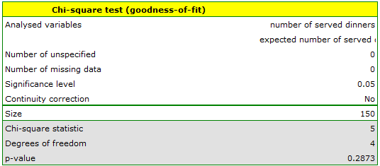
The p-value from the $\chi^2$ distribution with 4 degrees of freedom comes to 0.2873. So using the significance level $\alpha=0.05$ you can estimate that there is no reason to reject the null hypothesis that informs about the compatibility of the number of served dinners with the expected number of dinners served within the particular days.

Note!

If you want to make more comparisons within the framework of a one research, it is possible to use the Bonferroni correction⁶⁾. The correction is used to limit the size of I type error, if we compare the observed frequencies and the expected ones between particular days, for example:

Friday $\Longleftrightarrow$ Monday,

Friday $\Longleftrightarrow$ Tuesday,

Friday $\Longleftrightarrow$ Wednesday,

Friday $\Longleftrightarrow$ Thursday,

Provided that, the comparisons are made independently. The significance level $\alpha=0.05$ for each comparison must be calculated according to this correction using the following formula: $\alpha=\frac{0.05}{r}$ , where $r$ is the number of executed comparisons. The significance level for each comparison according to the Bonferroni correction (in this example) is $\alpha=\frac{0.05}{4}=0.0125$ .

However, it is necessary to remember that if you reduce $\alpha$ for each comparison, the power of the test is increased.

2022/02/09 12:56

Tests for one proportion

You should use tests for proportion if there are two possible results to obtain (one of them is an distinguished result with the size of m) and you know how often these results occur in the sample (we know a Z proportion). Depending on a sample size $n$ you can choose the Z test for a one proportion – for large samples and the exact binomial test for a one proportion – for small sample sizes . These tests are used to verify the hypothesis that the proportion in the population, from which the sample is taken, is a given value.

Basic assumptions:

measurement on a nominal scale - any order is not taken into account.

The additional condition for the Z test for proportion

large frequencies (according to Marascuilo and McSweeney interpretation (1977)⁷⁾ each of these values: $np>5$ and $n(1-p)>5$ ).

Hypotheses:

$\begin{array}{cl} \mathcal{H}_0: & p=p_0,\\ \mathcal{H}_1: & p\neq p_0, \end{array}$

where:

$p$ – probability (distinguished proportion) in the population,

$p_0$ – expected probability (expected proportion).

The Z test for one proportion

The test statistic is defined by:

$\begin{displaymath} Z=\frac{p-p_0}{\sqrt{\frac{p_0(1-p_0)}{n}}}, \end{displaymath}$

where:

$p=\frac{m}{n}$ distinguished proportion for the sample taken from the population,

$m$ – frequency of values distinguished in the sample,

$n$ – sample size.

The test statistic with a continuity correction is defined by:

$\begin{displaymath} Z=\frac{|p-p_0|-\frac{1}{2n}}{\sqrt{\frac{p_0(1-p_0)}{n}}}. \end{displaymath}$

The $Z$ statistic with and without a continuity correction asymptotically (for large sizes) has the normal distribution.

Binomial test for one proportion

The binomial test for one proportion uses directly the binomial distribution which is also called the Bernoulli distribution, which belongs to the group of discrete distributions (such distributions, where the analysed variable takes in the finite number of values). The analysed variable can take in $k=2$ values. The first one is usually definited with the name of a success and the other one with the name of a failure. The probability of occurence of a success (distinguished probability) is $p_0$ , and a failure $1-p_0$ .

The probability for the specific point in this distribution is calculated using the formula:

$\begin{displaymath} P(m)={n \choose m}p_0^m(1-p_0)^{n-m}, \end{displaymath}$

where:

${n \choose m}=\frac{n!}{m!(n-m)!}$ ,

$m$ – frequency of values distinguished in the sample,

$n$ – sample size.

Based on the total of appropriate probabilities $P$ a one-sided and a two-sided p-value is calculated, and a two-sided $p$ value is defined as a doubled value of the less of the one-sided probabilities.

The p-value is compared with the significance level $\alpha$ :

$\begin{array}{ccl} $ if $ p \le \alpha & \Longrightarrow & $ reject $ \mathcal{H}_0 $ and accept $ \mathcal{H}_1, \\ $ if $ p > \alpha & \Longrightarrow & $ there is no reason to reject $ \mathcal{H}_0. \\ \end{array}$

Note

Note that, for the estimator from the sample, which in this case is the value of the $p$ proportion, a confidence interval is calculated. The interval for a large sample size can be based on the normal distribution - so-called Wald intervals. The more universal are intervals proposed by Wilson (1927)⁸⁾ and by Agresti and Coull (1998)⁹⁾. Clopper and Pearson (1934)¹⁰⁾ intervals are more adequate for small sample sizes.

Comparison of interval estimation methods of a binomial proportion was published by Brown L.D et al (2001)¹¹⁾

The settings window with the Z test for one proportion can be opened in Statistics menu→NonParametric tests (unordered categories)→Z for proportion.

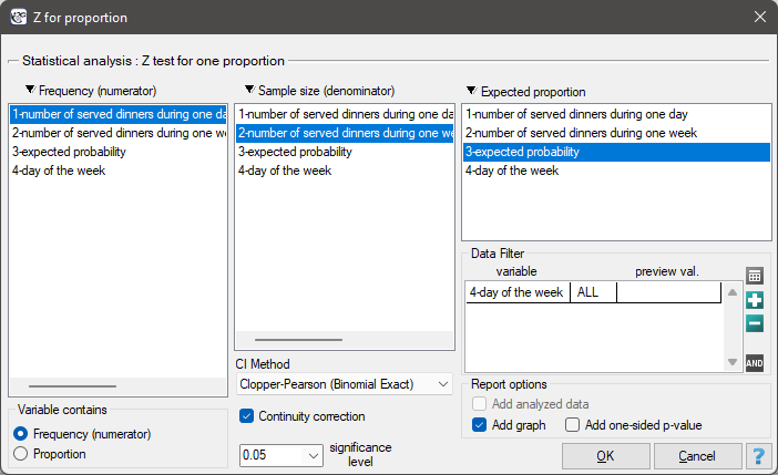
EXAMPLE cont. (dinners.pqs file)

Assume, that you would like to check if on Friday $\frac{1}{5}$ of all the dinners during the whole week are served. For the chosen sample $m=20$ , $n=150$ .

Select the options of the analysis and activate a filter selecting the appropriate day of the week – Friday. If you do not activate the filter, no error will be generated, only statistics for given weekdays will be calculated.

Hypotheses:

$\begin{array}{cl} \mathcal{H}_0: & $on Friday, in a school canteen there are served $\frac{1}{5}$ out of all dinners which are served$ \\ & $within a week,$\\ \mathcal{H}_1: & $on Friday, in a school canteen there are significantly more than $\frac{1}{5}$ or less than $\frac{1}{5} \\ & $dinners out of all the dinners served within a week in this canteen.$ \end{array}$

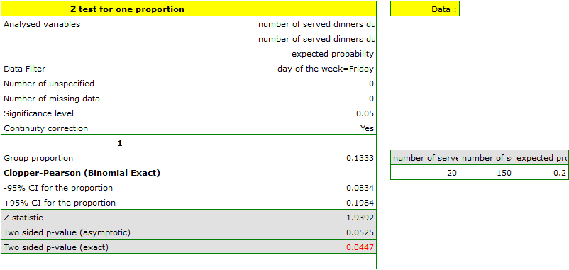
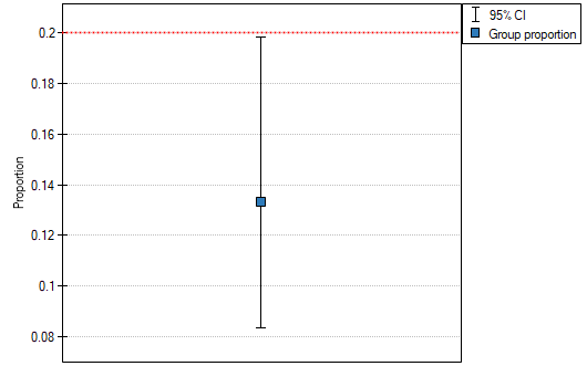
The proportion of the distinguished value in the sample is $p=\frac{m}{n}=0.133$ and 95% Clopper-Pearson confidence interval for this fraction $(0.083, 0.198)$ does not include the hypothetical value of 0.2.

Based on the Z test without the continuity correction (p-value = 0.0412) and also on the basis of the exact value of the probability calculated from the binomial distribution (p-value = 0.0447) you can assume (on the significance level $\alpha=0.05$ ), that on Friday there are statistically less than $\frac{1}{5}$ dinners served within a week. However, after using the continuity correction it is not possible to reject the null hypothesis p-value = 0.0525).

2022/02/09 12:56

¹⁾

Wilcoxon F. (1945), Individual comparisons by ranking methods. Biometries 1, 80-83

²⁾ , ⁷⁾

Marascuilo L.A. and McSweeney M. (1977), Nonparametric and distribution-free method for the social sciences. Monterey, CA: Brooks Cole Publishing Company

³⁾

Fritz C.O., Morris P.E., Richler J.J.(2012), Effect size estimates: Current use, calculations, and interpretation. Journal of Experimental Psychology: General., 141(1):2–18.

⁴⁾

Cohen J. (1988), Statistical Power Analysis for the Behavioral Sciences, Lawrence Erlbaum Associates, Hillsdale, New Jersey

⁵⁾

Cochran W.G. (1952), The chi-square goodness-of-fit test. Annals of Mathematical Statistics, 23, 315-345

⁶⁾

Abdi H. (2007), Bonferroni and Sidak corrections for multiple comparisons, in N.J. Salkind (ed.): Encyclopedia of Measurement and Statistics. Thousand Oaks, CA: Sage

⁸⁾

E.B. (1927), Probable Inference, the Law of Succession, and Statistical Inference. Journal of the American Statistical Association: 22(158):209-212

⁹⁾

Agresti A., Coull B.A. (1998), Approximate is better than „exact” for interval estimation of binomial proportions. American Statistics 52: 119-126

¹⁰⁾

Clopper C. and Pearson S. (1934), The use of confidence or fiducial limits illustrated in the case of the binomial. Biometrika 26: 404-413

¹¹⁾

Brown L.D., Cai T.T., DasGupta A. (2001), Interval Estimation for a Binomial Proportion. Statistical Science, Vol. 16, no. 2, 101-133

PQStat - Baza Wiedzy

Narzędzia użytkownika

Narzędzia witryny

Pasek boczny

Spis treści

Non-parametric tests

The Wilcoxon test (signed-ranks)

The Chi-square goodness-of-fit test

Tests for one proportion

Narzędzia strony