PQStat - Baza Wiedzy

Spis treści

Multiple Linear Regression

Multiple Linear Regression

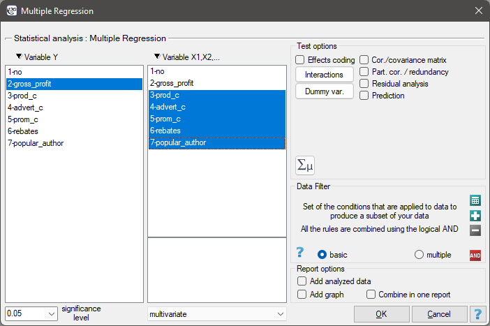
The window with settings for Multiple Regression is accessed via the menu Advanced statistics→Multidimensional Models→Multiple Regression

The constructed model of linear regression allows the study of the influence of many independent variables( $X_1,X_2,\ldots,X_k$ ) on one dependent variable( $Y$ ). The most frequently used variety of multiple regression is Multiple Linear Regression. It is an extension of linear regression models based on Pearson's linear correlation coefficient. It presumes the existence of a linear relation between the studied variables. The linear model of multiple regression has the form: $\begin{displaymath} Y=\beta_0+\beta_1X_1+\beta_2X_2+\ldots+\beta_kX_k+\epsilon. \end{displaymath}$

where:

$Y$ - dependent variable, explained by the model,

$X_1,X_2,\ldots X_k$ - independent variables, explanatory,

$\beta_0,\beta_1,\beta_2,\ldots \beta_k$ - parameters,

$\epsilon$ - random parameter (model residual).

If the model was created on the basis of a data sample of size $n$ the above equation can be presented in the form of a matrix: $\begin{displaymath} Y=X\beta+\epsilon. \end{displaymath}$

where:

$Y=\left( \begin{array}{ccc} y_1\\ y_2\\ \vdots\\ y_n \end{array} \right),$

$X=\left( \begin{array}{ccccc} 1 & x_{11} & x_{21} & \ldots & x_{k1}\\ 1 & x_{12} & x_{22} & \ldots & x_{k2}\\ \vdots & \vdots & \vdots & \ddots & \vdots\\ 1 & x_{1n} & x_{2n} & \ldots & x_{kn} \end{array}\right),$

$\beta=\left( \begin{array}{ccc} \beta_0\\ \beta_1\\ \beta_2\\ \vdots\\ \beta_k \end{array} \right),$

$\epsilon=\left(\begin{array}{ccc} \epsilon_1\\ \epsilon_2\\ \vdots\\ \epsilon_n \end{array} \right).$

In such a case, the solution of the equation is the vector of the estimates of parameters $\beta_0,\beta_1,\ldots,\beta_k$ called regression coefficients:

$b=\left( \begin{array}{ccc} b_0\\ b_1\\ b_2\\ \vdots\\ b_k \end{array} \right).$

Those coefficients are estimated with the help of the classical least squares method. On the basis of those values we can infer the magnitude of the effect of the independent variable (for which the coefficient was estimated) on the dependent variable. They inform by how many units will the dependent variable change when the independent variable is changed by 1 unit. There is a certain error of estimation for each coefficient. The magnitude of that error is estimated from the following formula:

$\begin{displaymath} SE_b=\sqrt{\frac{1}{n-(k+1)}e^Te(X^TX)^{-1}}, \end{displaymath}$

where:

$e=Y-\widehat{Y}$ is the vector of model residuals (the difference between the actual values of the dependent variable Y and the values $\widehat{Y}$ predicted on the basis of the model).

Dummy variables and interactions in the model

A discussion of the coding of dummy variables and interactions is presented in chapter Preparation of the variables for the analysis in multidimensional models.

Note When constructing the model one should remember that the number of observations should meet the assumptions ( $n\ge 50 +8k$ ) where $k$ is the number of explanatory variables in the model ¹⁾.

Model verification

Statistical significance of particular variables in the model.

On the basis of the coefficient and its error of estimation we can infer if the independent variable for which the coefficient was estimated has a significant effect on the dependent variable. For that purpose we use t-test.

Hypotheses:

$\begin{array}{cc} \mathcal{H}_0: & \beta_i=0,\\ \mathcal{H}_1: & \beta_i\ne 0. \end{array}$

Let us estimate the test statistics according to the formula below:

$\begin{displaymath} t=\frac{b_i}{SE_{b_i}} \end{displaymath}$

The test statistics has t-Student distribution with $n-k$ degrees of freedom.

The p-value, designated on the basis of the test statistic, is compared with the significance level $\alpha$ :

$\begin{array}{ccl} $ if $ p \le \alpha & \Longrightarrow & $ reject $ \mathcal{H}_0 $ and accept $ \mathcal{H}_1, \\ $ if $ p > \alpha & \Longrightarrow & $ there is no reason to reject $ \mathcal{H}_0. \\ \end{array}$

The quality of the constructed model of multiple linear regression can be evaluated with the help of several measures.

The standard error of estimation – it is the measure of model adequacy:

$\begin{displaymath} SE_e=\sqrt{\frac{\sum_{i=1}^ne_i^2}{n-(k+1)}}. \end{displaymath}$

The measure is based on model residuals $e_i=y_i-\widehat{y}_i$ , that is on the discrepancy between the actual values of the dependent variable $y_i$ in the sample and the values of the independent variable $\widehat{y}_i$ estimated on the basis of the constructed model. It would be best if the difference were as close to zero as possible for all studied properties of the sample. Therefore, for the model to be well-fitting, the standard error of estimation ( $SE_e$ ), expressed as $e_i$ variance, should be the smallest possible.

Multiple correlation coefficient $R=\sqrt{R^2} \in <0; 1>$ – defines the strength of the effect of the set of variables $X_1,X_2,\ldots X_k$ on the dependent variable $Y$ .
Multiple determination coefficient $R^2$ – it is the measure of model adequacy.

The value of that coefficient falls within the range of $<0; 1>$ , where 1 means excellent model adequacy, 0 – a complete lack of adequacy. The estimation is made using the following formula:

$\begin{displaymath} T_{SS}=E_{SS}+R_{SS}, \end{displaymath}$

where:

$T_{SS}$ – total sum of squares,

$E_{SS}$ – the sum of squares explained by the model,

$R_{SS}$ – residual sum of squares.

The coefficient of determination is estimated from the formula:

$\begin{displaymath} R^2=\frac{T_{SS}}{E_{SS}}. \end{displaymath}$

It expresses the percentage of the variability of the dependent variable explained by the model.

As the value of the coefficient $R^2$ depends on model adequacy but is also influenced by the number of variables in the model and by the sample size, there are situations in which it can be encumbered with a certain error. That is why a corrected value of that parameter is estimated:

$\begin{displaymath} R^2_{adj}=R^2-\frac{k(1-R^2)}{n-(k+1)}. \end{displaymath}$

Information criteria are based on the entropy of information carried by the model (model uncertainty) i.e. they estimate the information lost when a given model is used to describe the phenomenon under study. Therefore, we should choose the model with the minimum value of a given information criterion.

The $AIC$ , $AICc$ and $BIC$ is a kind of trade-off between goodness of fit and complexity. The second element of the sum in the information criteria formulas (the so-called loss or penalty function) measures the simplicity of the model. It depends on the number of variables in the model ( $k$ ) and the sample size ( $n$ ). In both cases, this element increases as the number of variables increases, and this increase is faster the smaller the number of observations.The information criterion, however, is not an absolute measure, i.e., if all the models being compared misdescribe reality in the information criterion there is no point in looking for a warning.

Akaike information criterion

$\begin{displaymath} AIC=n\cdot \ln{\frac{R_{SS}}{n}}+2(k+1)+(constant) \end{displaymath}$

where, the constant can be omitted because it is the same in each of the compared models.

This is an asymptotic criterion - suitable for large samples i.e. when $\frac{n}{k+2}>40$ . For small samples, it tends to favor models with a large number of variables.

Example of interpretation of AIC size comparison

Suppose we determined the AIC for three models $AIC_1$ =100, $AIC_2$ =101.4, $AIC_3$ =110. Then the relative reliability for the model can be determined. This reliability is relative because it is determined relative to another model, usually the one with the smallest AIC value. We determine it according to the formula: $e^{(AIC_{min}− AIC_i)/2}$ . Comparing model 2 to model 1, we will say that the probability that it will minimize the loss of information is about half of the probability that model 1 will do so (specifically exp((100− 101.4)/2) = 0.497). Comparing model 3 to model one, we will say that the probability that it will minimize information loss is a small fraction of the probability that model 1 will do so (specifically exp((100- 110)/2) = 0.007).

Akaike coreccted information criterion

$\begin{displaymath} AICc=AIC+\frac{2(k+3)(k+4)}{n-k} \end{displaymath}$

Correction of Akaike's criterion relates to sample size, which makes this measure recommended also for small sample sizes.

Bayes Information Criterion (or Schwarz criterion)

$\begin{displaymath} BIC=n\cdot \ln{\frac{R_{SS}}{n}}+(k+1)\ln{n}+(constant) \end{displaymath}$

where, the constant can be omitted because it is the same in each of the compared models.

Like Akaike's revised criterion, the BIC takes into account the sample size.

Error analysis for ex post forecasts:

MAE (mean absolute error) -– forecast accuracy specified by MAE informs how much on average the realised values of the dependent variable will deviate (in absolute value) from the forecasts.

$\begin{displaymath} MAE=\frac{1}{n}\sum_{i=1}^n\left|e_i\right| \end{displaymath}$

MPE (mean percentage error) -– informs what average percentage of the realization of the dependent variable are forecast errors.

$\begin{displaymath} MPE=\frac{1}{n}\sum_{i=1}^n\frac{e_i}{y_i} \end{displaymath}$

MAPE (mean absolute percentage error) -– informs about the average size of forecast errors expressed as a percentage of the actual values of the dependent variable. MAPE allows you to compare the accuracy of forecasts obtained from different models.

$\begin{displaymath} MAPE=\frac{1}{n}\sum_{i=1}^n\left|\frac{e_i}{y_i}\right| \end{displaymath}$

Statistical significance of all variables in the model

The basic tool for the evaluation of the significance of all variables in the model is the analysis of variance test (the F-test). The test simultaneously verifies 3 equivalent hypotheses:

$\begin{array}{cc} \mathcal{H}_0: & \textrm{all }\beta_i=0,\\ \mathcal{H}_0: & R^2=0,\\ \mathcal{H}_0: & $linearity of the relation$, \end{array}$ $\begin{array}{cc} \mathcal{H}_1: & \textrm{exists } \beta_i\neq0;\\ \mathcal{H}_1: & R^2\neq0;\\ \mathcal{H}_1: & $a lack of a linear relation$. \end{array}$

The test statistics has the form presented below:

$\begin{displaymath} F=\frac{E_{MS}}{R_{MS}} \end{displaymath}$

where:

$\displaystyle E_{MS}=\frac{E_{SS}}{df_{E}}$ – the mean square explained by the model,

$\displaystyle R_{MS}=\frac{R_{SS}}{df_{R}}$ – residual mean square,

$df_E=k$ , $df_R=n-(k+1)$ – appropriate degrees of freedom.

That statistics is subject to F-Snedecor distribution with $df_E$ and $df_R$ degrees of freedom.

The p-value, designated on the basis of the test statistic, is compared with the significance level $\alpha$ :

$\begin{array}{ccl} $ if $ p \le \alpha & \Longrightarrow & $ reject $ \mathcal{H}_0 $ and accept $ \mathcal{H}_1, \\ $ if $ p > \alpha & \Longrightarrow & $ there is no reason to reject $ \mathcal{H}_0. \\ \end{array}$

EXAMPLE (publisher.pqs file)

2022/02/09 12:56

More information about the variables in the model

* Standardized $b_1,b_2,\ldots,b_k$ – In contrast to raw parameters (which are expressed in different units of measure, depending on the described variable, and are not directly comparable) the standardized estimates of the parameters of the model allow the comparison of the contribution of particular variables to the explanation of the variance of the dependent variable $Y$ .

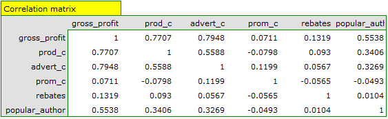
Correlation matrix – contains information about the strength of the relation between particular variables, that is the Pearson's correlation coefficient $r_p \in <-1; 1>$ . The coefficient is used for the study of the corrrelation of each pair of variables, without taking into consideration the effect of the remaining variables in the model.
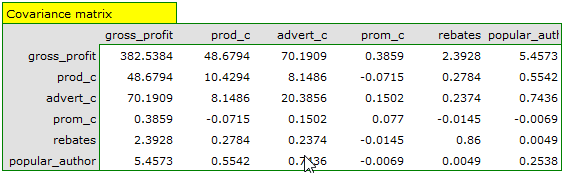
Covariance matrix – similarly to the correlation matrix it contains information about the linear relation among particular variables. That value is not standardized.
Partial correlation coefficient – falls within the range $<-1; 1>$ and is the measure of correlation between the specific independent variable $X_i$ (taking into account its correlation with the remaining variables in the model) and the dependent variable $Y$ (taking into account its correlation with the remaining variables in the model).

The square of that coefficient is the partial determination coefficient – it falls within the range $<0; 1>$ and defines the relation of only the variance of the given independent variable $X_i$ with that variance of the dependent variable $Y$ which was not explained by other variables in the model.

The closer the value of those coefficients to 0, the more useless the information carried by the studied variable, which means the variable is redundant.

Semipartial correlation coefficient – falls within the range $<-1; 1>$ and is the measure of correlation between the specific independent variable $X_i$ (taking into account its correlation with the remaining variables in the model) and the dependent variable $Y$ (NOT taking into account its correlation with the remaining variables in the model).

The square of that coefficient is the semipartial determination coefficient – it falls within the range $<0; 1>$ and defines the relation of only the variance of the given independent variable $X_i$ with the complete variance of the dependent variable $Y$ .

The closer the value of those coefficients to 0, the more useless the information carried by the studied variable, which means the variable is redundants.

R-squared ( $R^2 \in <0; 1>$ ) – it represents the percentage of variance of the given independent variable $X_i$ , explained by the remaining independent variables. The closer to value 1 the stronger the linear relation of the studied variable with the remaining independent variables, which can mean that the variable is a redundant one.
Variance inflation factor ( $VIF \in <1; \infty )$ ) – determines how much the variance of the estimated regression coefficient is increased due to collinearity. The closer the value is to 1, the lower the collinearity and the smaller its effect on the coefficient variance. It is assumed that strong collinearity occurs when the coefficient VIF>5 \cite{sheather}. f the variance inflation factor is 5 ( $\sqrt{5}$ = 2.2), this means that the standard error for the coefficient of this variable is 2.2 times larger than if this variable had zero correlation with other variables $X_i$ .
Tolerance = $1-R^2 \in<0; 1>$ – it represents the percentage of variance of the given independent variable $X_i$ , NOT explained by the remaining independent variables. The closer the value of tolerance is to 0 the stronger the linear relation of the studied variable with the remaining independent variables, which can mean that the variable is a redundant one.
A comparison of a full model with a model in which a given variable is removed

The comparison of the two model is made with by means of:

F test, in a situation in which one variable or more are removed from the model (see: the comparison of models),
t-test, when only one variable is removed from the model. It is the same test that is used for studying the significance of particular variables in the model.

In the case of removing only one variable the results of both tests are identical.

If the difference between the compared models is statistically significant (the value $p \le \alpha$ ), the full model is significantly better than the reduced model. It means that the studied variable is not redundant, it has a significant effect on the given model and should not be removed from it.

Scatter plots

The charts allow a subjective evaluation of linearity of the relation among the variables and an identification of outliers. Additionally, scatter plots can be useful in an analysis of model residuals.

2022/02/09 12:56

Analysis of model residuals

To obtain a correct regression model we should check the basic assumptions concerning model residuals.

Outliers

The study of the model residual can be a quick source of knowledge about outlier values. Such observations can disturb the equation of the regression to a large extent because they have a great effect on the values of the coefficients in the equation. If the given residual $e_i$ deviates by more than 3 standard deviations from the mean value, such an observation can be classified as an outlier. A removal of an outlier can greatly enhance the model.

Cook's distance - describes the magnitude of change in regression coefficients produced by omitting a case. In the program, Cook's distances for cases that exceed the 50th percentile of the F-Snedecor distribution statistic are highlighted in bold $F(0.5, k+1, n-k-1)$ .

Mahalanobis distance - is dedicated to detecting outliers - high values indicate that a case is significantly distant from the center of the independent variables. If a case with the highest Mahalanobis value is found among the cases more than 3 deviations away, it will be marked in bold as the outlier.

Normalność rozkładu reszt modelu

We check this assumption visually using a Q-Q plot of the nromal distribution. The large difference between the distribution of the residuals and the normal distribution may disturb the assessment of the significance of the coefficients of the individual variables in the model.

Homoscedasticity (homogeneity of variance)

To check if there are areas in which the variance of model residuals is increased or decreased we use the charts of:

the residual with respect to predicted values
the square of the residual with respect to predicted values
the residual with respect to observed values
the square of the residual with respect to observed values

Autocorrelation of model residuals

For the constructed model to be deemed correct the values of residuals should not be correlated with one another (for all pairs $e_i, e_j$ ). The assumption can be checked by by computing the Durbin-Watson statistic.

$\begin{displaymath} d=\frac{\sum_{t=2}^n\left(e_t-e_{t-1}\right)^2}{\sum_{t=1}^ne_t^2}, \end{displaymath}$

To test for positive autocorrelation on the significance level $\alpha$ we check the position of the statistics $d$ with respect to the upper ( $d_{U,\alpha}$ ) and lower ( $d_{L,\alpha}$ ) critical value:

If $d <d_{L,\alpha}$ – the errors are positively correlated;
If $d> d_{U,\alpha}$ – the errors are not positively correlated;
If $d_{L,\alpha}<d <d_{U,\alpha}$ – the test result is ambiguous.

To test for negative autocorrelation on the significance level $\alpha$ we check the position of the value $4-d$ with respect to the upper ( $d_{U,\alpha}$ ) and lower ( $d_{L,\alpha}$ ) critical value:

If $4-d <d_{L,\alpha}$ – the errors are negatively correlated;
If $4-d> d_{U,\alpha}$ – the errors are not negatively correlated;
If $d_{L,\alpha}<4-d <d_{U,\alpha}$ – the test result is ambiguous.

The critical values of the Durbin-Watson test for the significance level $\alpha=0.05$ are on the website (pqstat) – the source of the: Savin and White tables (1977)²⁾

EXAMPLE cont. (publisher.pqs file)

2022/02/09 12:56

Example for multiple regression

EXAMPLE (publisher.pqs file)

A certain book publisher wanted to learn how was gross profit from sales influenced by such variables as: production cost, advertising costs, direct promotion cost, the sum of discounts made, and the author's popularity. For that purpose he analyzed 40 titles published during the previous year (teaching set). A part of the data is presented in the image below:

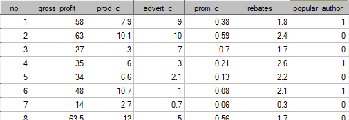
The first five variables are expressed in thousands fo dollars - so they are variables gathered on an interval scale. The last variable: the author's popularity – is a dychotomic variable, where 1 stands for a known author, and 0 stands for an unknown author.

On the basis of the knowledge gained from the analysis the publisher wants to predict the gross profit from the next published book written by a known author. The expenses the publisher will bear are: production cost $\approx 11$ , advertising costs $\approx 13$ , direct promotion costs $\approx 0.5$ , the sum of discounts made $\approx 0.5$ .

We construct the model of multiple linear regression, for teaching dataset, selecting: gross profit – as the dependent variable $Y$ , production cost, advertising costs, direct promotion costs, the sum of discounts made, the author's popularity – as the independent variables $X_1, X_2, X_3, X_4, X_5$ . As a result, the coefficients of the regression equation will be estimated, together with measures which will allow the evaluation of the quality of the model.

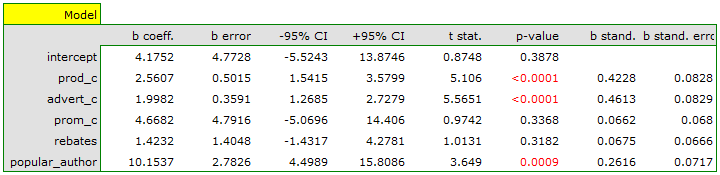
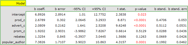
On the basis of the estimated value of the coefficient $b$ , the relationship between gross profit and all independent variables can be described by means of the equation: $\begin{displaymath} profit_{gross}=4.18+2.56(c_{prod})+2(c_{adv})+4.67(c_{prom})+1.42(discounts)+10.15(popul_{author})+[8.09] \end{displaymath}$ The obtained coefficients are interpreted in the following manner:

If the production cost increases by 1 thousand dollars, then gross profit will increase by about 2.56 thousand dollars, assuming that the remaining variables do not change;
If the production cost increases by 1 thousand dollars, then gross profit will increase by about 2 thousand dollars, assuming that the remaining variables do not change;
If the production cost increases by 1 thousand dollars, then gross profit will increase by about 4.67 thousand dollars, assuming that the remaining variables do not change;
If the sum of the discounts made increases by 1 thousand dollars, then gross profit will increase by about 1.42 thousand dollars, assuming that the remaining variables do not change;
If the book has been written by a known author (marked as 1), then in the model the author's popularity is assumed to be the value 1 and we get the equation:

$\begin{displaymath} profit_{gross}=14.33+2.56(c_{prod})+2(c_{adv})+4.67(c_{prom})+1.42(discounts) \end{displaymath}$

If the book has been written by an unknown author (marked as 0), then in the model the author's popularity is assumed to be the value 0 and we get the equation: $\begin{displaymath} profit_{gross}=4.18+2.56(c_{prod})+2(c_{adv})+4.67(c_{prom})+1.42(discounts) \end{displaymath}$

The result of t-test for each variable shows that only the production cost, advertising costs, and author's popularity have a significant influence on the profit gained. At the same time, that standardized coefficients $b$ are the greatest for those variables.

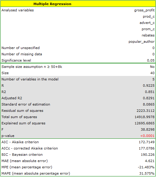
Additionally, the model is very well-fitting, which is confirmed by: the small standard error of estimation $SE_e=8.087$ , the high value of the multiple determination coefficient $R^2=0.85$ , the corrected multiple determination coefficient $R_{adj}^2= 0.83$ , and the result of the F-test of variance analysis: p<0.0001.

On the basis of the interpretation of the results obtained so far we can assume that a part of the variables does not have a significant effect on the profit and can be redundant. For the model to be well formulated the interval independent variables ought to be strongly correlated with the dependent variable and be relatively weakly correlated with one another. That can be checked by computing the correlation matrix and the covariance matrix:

The most coherent information which allows finding those variables in the model which are redundant is given by the parial and semipartial correlation analysis as well as redundancy analysis:

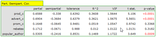
The values of coefficients of partial and semipartial correlation indicate that the smallest contribution into the constructed model is that of direct promotion costs and the sum of discounts made. However, those variables are the least correlated with model residuals, which is indicated by the low value $R^2$ and the high tolerance value. All in all, from the statistical point of view, models without those variables would not be worse than the current model (see the result of t-test for model comparison). The decision about whether or not to leave that model or to construct a new one without the direct promotion costs and the sum of discounts made, belongs to the researcher. We will leave the current model.

Finally, we will analyze the residuals. A part of that analysis is presented below:

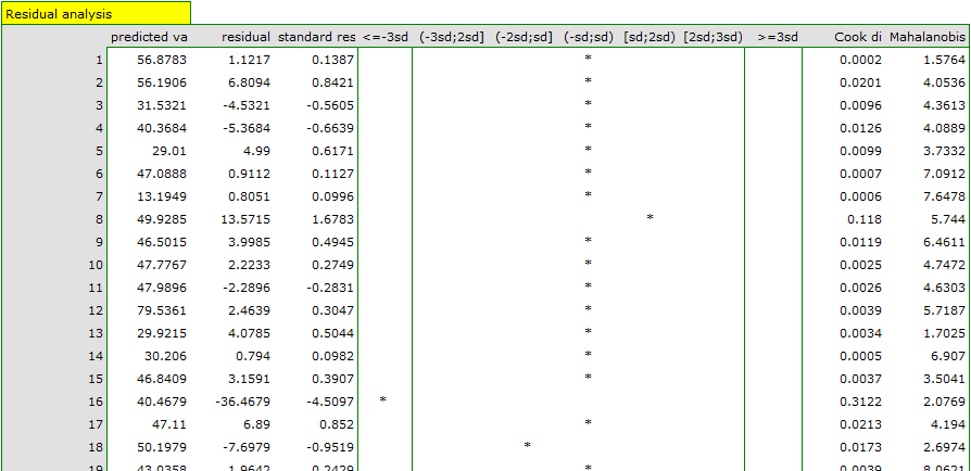
It is noticeable that one of the model residuals is an outlier – it deviates by more than 3 standard deviations from the mean value. It is observation number 16. The observation can be easily found by drawing a chart of residuals with respect to observed or expected values of the variable $Y$ .

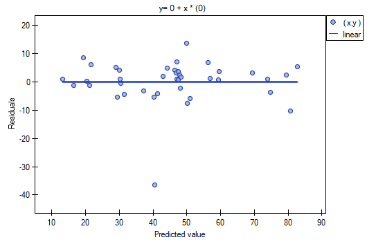
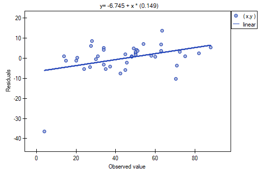
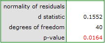
That outlier undermines the assumption concerning homoscedasticity. The assumption of homoscedasticity would be confirmed (that is, residuals variance presented on the axis $Y$ would be similar when we move along the axis $X$ ), if we rejected that point. Additionally, the distribution of residuals deviates slightly from normal distribution (the value $p$ of Liliefors test is p=0.0164):

When we take a closer look of the outlier (position 16 in the data for the task) we see that the book is the only one for which the costs are higher than gross profit (gross profit=4 thousand dollars, the sum of costs = (8+6+0.33+1.6) = 15.93 thousand dollars).

The obtained model can be corrected by removing the outlier. For that purpose, another analysis has to be conducted, with a filter switched on which will exclude the outlier.

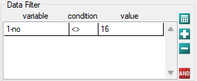
As a result, we receive a model which is very similar to the previous one but is encumbered with a smaller error and is more adequate:

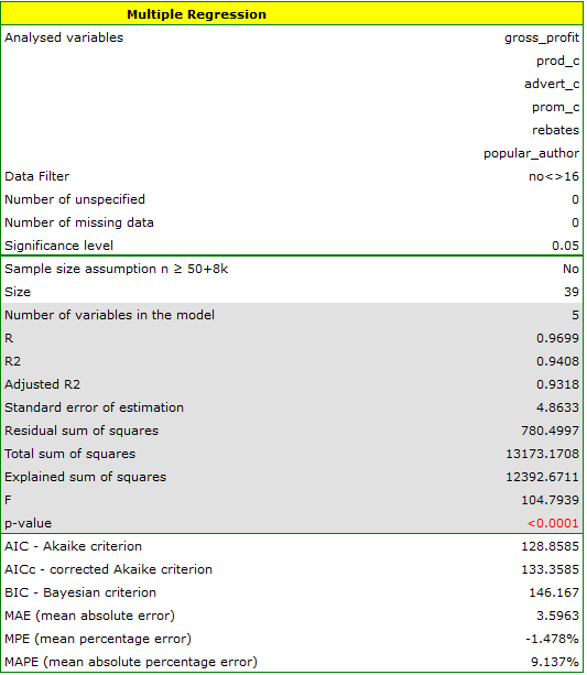
$\begin{displaymath} profit_{gross}=6.89+2.68(c_{prod})+2.08(c_{adv})+1.92(c_{prom})+1.33(discounts)+7.38(popul_{author})+[4.86] \end{displaymath}$

The final version of the model will be used for prediction. On the basis of the predicted costs amounting to: production cost $\approx 11$ thousand dollars,\\advertising costs $\approx 13$ thousand dollars,\\direct promotion costs $\approx 0.5$ thousand dollars,\\the sum of discounts made $\approx 0.5$ thousand dollars,\\and the fact that the author is known (the author's popularity $\approx 1$ ) we calculate the predicted gross profit together with the confidence interval:

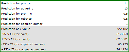
The predicted profit is 72 thousand dollars.

Finally, it should still be noted that this is only a preliminary model. In a proper study more data would have to be collected. The number of variables in the model is too small in relation to the number of books evaluated, i.e. n<50+8k.

2022/02/09 12:56

Model-based prediction and test set validation

Validation

Validation of a model is a check of its quality. It is first performed on the data on which the model was built (the so-called training data set), that is, it is returned in a report describing the resulting model. In order to be able to judge with greater certainty how suitable the model is for forecasting new data, an important part of the validation is to become a model to data that were not used in the model estimation. If the summary based on the treining data is satisfactory, i.e., the determined errors $R^2$ coefficients and information criteria are at a satisfactory level, and the summary based on the new data (the so-called test data set) is equally favorable, then with high probability it can be concluded that such a model is suitable for prediction. The testing data should come from the same population from which the training data were selected. It is often the case that before building a model we collect data, and then randomly divide it into a training set, i.e. the data that will be used to build the model, and a test set, i.e. the data that will be used for additional validation of the model.

The settings window with the validation can be opened in Advanced statistics→Multivariate models→Multiple regression - prediction/validation.

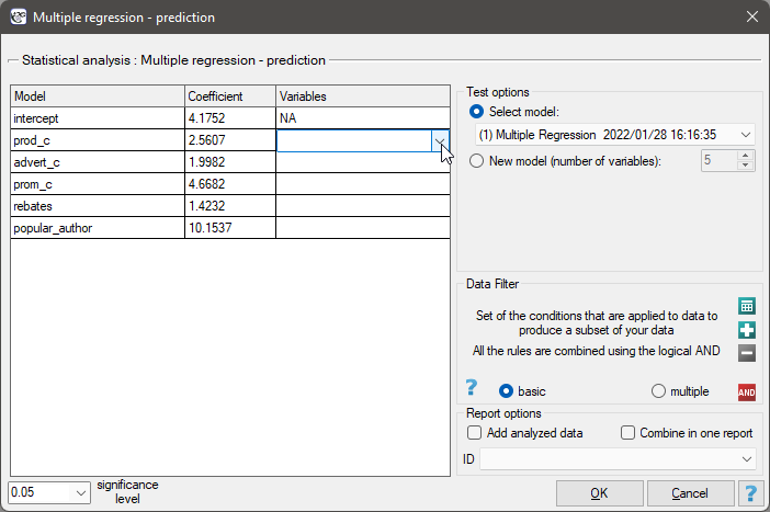
To perform validation, it is necessary to indicate the model on the basis of which we want to perform the validation. Validation can be done on the basis of:

multivariate regression model built in PQStat - simply select a model from the models assigned to the sheet, and the number of variables and model coefficients will be set automatically; the test set should be in the same sheet as the training set;
model not built in PQStat but obtained from another source (e.g., described in a scientific paper we have read) - in the analysis window, enter the number of variables and enter the coefficients for each of them.

In the analysis window, indicate those new variables that should be used for validation.

Prediction

Most often, the final step in regression analysis is to use the built and previously validated model for prediction.

Prediction for a single object can be performed along with the construction of the model, that is, in the analysis window Advanced statistics→Multivariate models→Multiple regression ,
Prediction for a larger group of new data is done through the menu Advanced statistics→Multivariate models→Multiple regression - prediction/validation.

To make a prediction, it is necessary to indicate the model on the basis of which we want to make the prediction. Prediction can be made on the basis of:

multivariate regression model built in PQStat -simply select a model from the models assigned to the sheet, and the number of variables and model coefficients will be set automatically; the test set should be in the same sheet as the training set;
model not built in PQStat but obtained from another source (e.g., described in a scientific paper we read) - in the analysis window, the number of variables and the coefficients on each of them should be entered.

In the analysis window, indicate those new variables that should be used for prediction. The estimated value is calculated with some error. Therefore, in addition, for the value predicted by the model, limits are set due to the error:

confidence intervals are set for the expected value,
For a single point, prediction intervals are determined.

Example continued (publisher.pqs file)

To predict gross profit from book sales, the publisher built a regression model based on a training set stripped of item 16 (that is, 39 books). The model included: production costs, advertising costs and author popularity (1=popular author, 0=not). We will build the model once again based on the learning set and then, to make sure the model will work properly, we will validate it on a test data set. If the model passes this test, we will apply it to predictions for book items. To use the right collections we set a data filter each time.

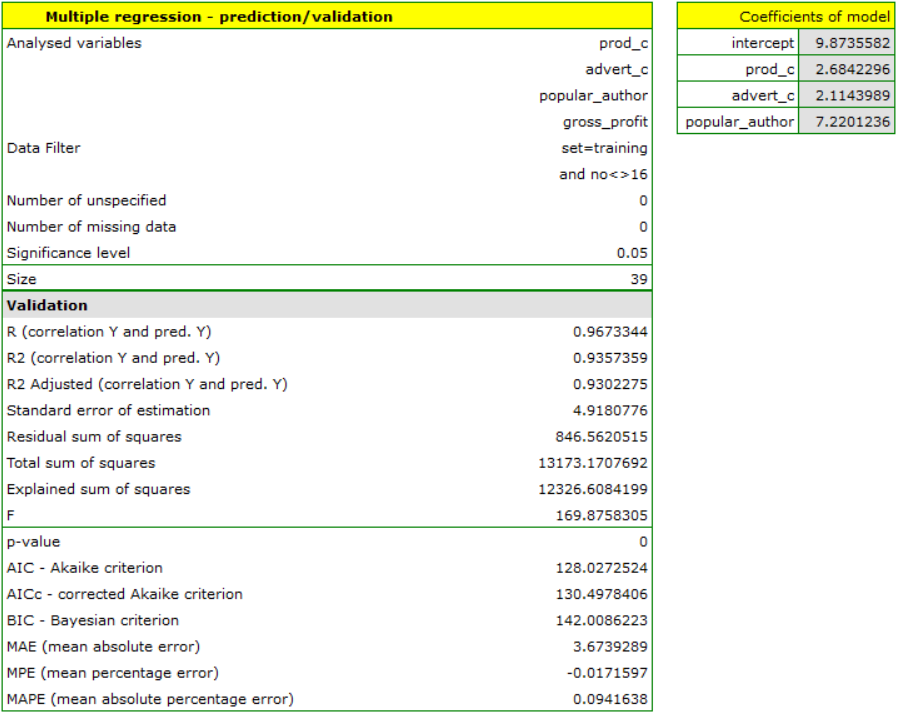
For the training set, the values describing the quality of the model's fit are very high: adjusted $R^2$ = 0.93 and the average forecast error (MAE) is 3.7 thousand dollars.

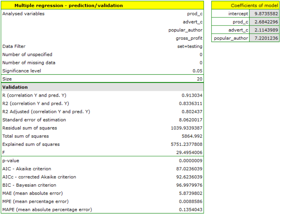
For the test set, the values describing the quality of the model fit are slightly lower than for the learning set: Adjusted $R^2$ = 0.80 and the mean error of prediction (MAE) is 5.9 thousand dollars. Since the validation result on the test set is almost as good as on the training set, we will use the model for prediction. To do this, we will use the data of three new book items added to the end of the set. We'll select Prediction, set filter on the new dataset and use our model to predict the gross profit for these books.

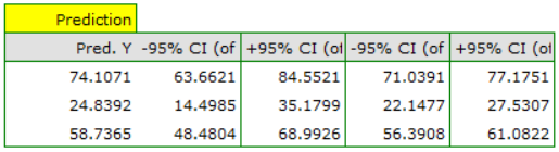
It turns out that the highest gross profit (between 64 and 85 thousands of dollars) is projected for the first, most advertised and most expensive book published by a popular author.

2022/02/09 12:56

¹⁾

Green, S.B. (1991), How many subjects does it take to do a regression analysis? Multivariate Behavioral Research, 26, 499-510

²⁾

Savin N.E. and White K.J. (1977), The Durbin-Watson Test for Serial Correlation with Extreme Sample Sizes or Many Regressors. Econometrica 45, 1989-1996

PQStat - Baza Wiedzy

Narzędzia użytkownika

Narzędzia witryny

Pasek boczny

Spis treści

Multiple Linear Regression

Model verification

More information about the variables in the model

Analysis of model residuals

Example for multiple regression

Model-based prediction and test set validation

Narzędzia strony