PQStat - Baza Wiedzy

Spis treści

Parametric tests
- The t-test for a single sample
- The Single-Sample Chi-square Test for a Population Variance

Parametric tests

The t-test for a single sample

The single-sample $t$ test is used to verify the hypothesis, that an analysed sample with the mean ( $\overline{x}$ ) comes from a population, where mean ( $\mu$ ) is a given value.
Basic assumptions:

measurement on an interval scale,
normality of distribution of an analysed feature.

Hypotheses:

$\begin{array}{cc} \mathcal{H}_0: & \mu=\mu_0,\\ \mathcal{H}_1: & \mu\ne \mu_0, \end{array}$

where:

$\mu$ – mean of an analysed feature of the population represented by the sample,

$\mu_0$ – a given value.

The test statistic is defined by: $\begin{displaymath} t=\frac{\overline{x}-\mu_0}{sd}\sqrt{n}, \end{displaymath}$

where:

$sd$ – standard deviation from the sample,

$n$ – sample size.

The test statistic has the t-Student distribution with $n-1$ degrees of freedom.

The p-value, designated on the basis of the test statistic, is compared with the significance level $\alpha$ :

$\begin{array}{ccl} $ if $ p \le \alpha & \Longrightarrow & $ reject $ \mathcal{H}_0 $ and accept $ \mathcal{H}_1, \\ $ if $ p > \alpha & \Longrightarrow & $ there is no reason to reject $ \mathcal{H}_0. \\ \end{array}$

Note

Note, that: If the sample is large and you know a standard deviation of the population, then you can calculate a test statistic using the formula: $\begin{displaymath} t=\frac{\overline{x}-\mu_0}{\sigma}\sqrt n. \end{displaymath}$ The statistic calculated this way has the normal distribution. If $n \rightarrow \infty$ $t$ -Student distribution converges to the normal distribution $N(0,1)$ . In practice, it is assumed, that with $n>30$ the $t$ -Student distribution may be approximated with the normal distribution.

Standardized effect size.

The Cohen's d determines how much of the variation occurring is the difference between the averages.

$\begin{displaymath} d=\left|\frac{\overline{x}-\mu_0}{sd}\right| \end{displaymath}$ .

When interpreting an effect, researchers often use general guidelines proposed by Cohen ¹⁾ defining small (0.2), medium (0.5) and large (0.8) effect sizes.

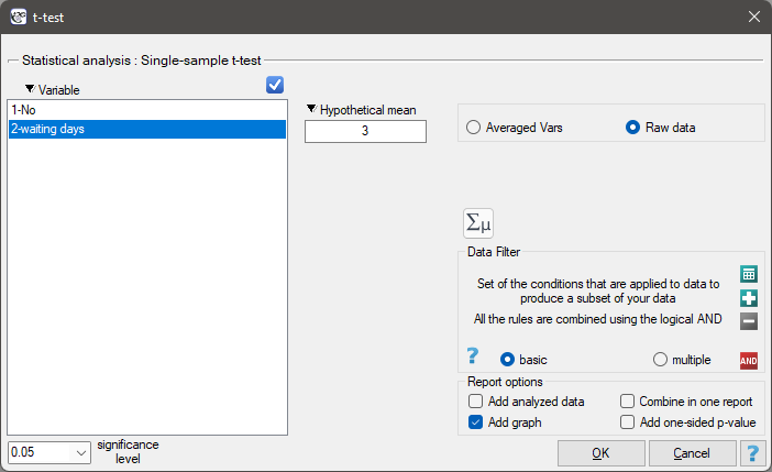
The settings window with the Single-sample <latex>$t$</latex>-test can be opened in Statistics menu→Parametric tests→t-test or in ''Wizard''.

Note

Calculations can be based on raw data or data that are averaged like: arithmetic mean, standard deviation and sample size.

EXAMPLE (courier.pqs file)

You want to check if the time of awaiting for a delivery by some courier company is 3 days on the average $(\mu_0=3)$ . In order to calculate it, there are 22 persons chosen by chance from all clients of the company as a sample. After that, there are written information about the number of days passed since the delivery was sent till it is delivered. There are following values: (1, 1, 1, 2, 2, 2, 2, 3, 3, 3, 4, 4, 4, 4, 4, 5, 5, 6, 6, 6, 7, 7).

The number of awaiting days for the delivery in the analysed population fulfills the assumption of normality of distribution.

Hypotheses:

$\begin{array}{cl} \mathcal{H}_0: & $mean of the number of awaiting days for the delivery, which is supposed$\\ &$to be delivered by the above-mentioned courier company is 3,$\\ \mathcal{H}_1: & $mean of the number of awaiting days for the delivery, which is supposed$\\ &$ to be delivered by the above-mentioned courier company is different from 3.$ \end{array}$

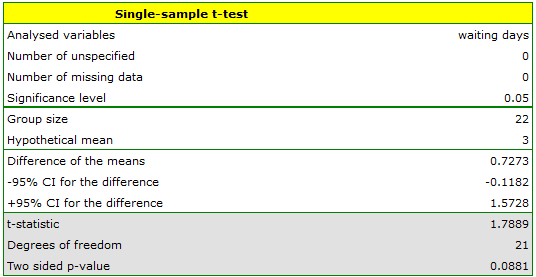
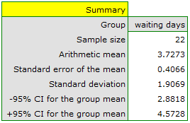
Comparing the $p$ value = 0.0881 of the $t$ -test with the significance level $\alpha=0.05$ we draw the conclusion, that there is no reason to reject the null hypothesis which informs that the average time of awaiting for the delivery, which is supposed to be delivered by the analysed courier company is 3. For the tested sample, the mean is $\overline{x}=3.73$ and the standard deviation is $sd=1.91$ .

2022/02/09 12:56

The Single-Sample Chi-square Test for a Population Variance

Basic assumptions:

measurement on an interval scale,
normality of distribution of an analysed feature.

Hypotheses:

$\begin{array}{cc} \mathcal{H}_0: & \sigma=\sigma_0,\\ \mathcal{H}_1: & \sigma\ne \sigma_0, \end{array}$

where:

$\sigma$ – standard deviation of a characteristic in the population represented by the sample,

$\sigma_0$ – setpoint.

The test statistic is defined by: $\begin{displaymath} t=\frac{(n-1)sd^2}{\sigma_0^2}, \end{displaymath}$

where:

$sd$ – standard deviation in the sample,

$n$ – sample size.

The test statistic has the Chi-square distribution with the degrees of freedom determined by the formula: $df=n-1$ .

The p-value, designated on the basis of the test statistic, is compared with the significance level $\alpha$ :

$\begin{array}{ccl} $ if $ p \le \alpha & \Longrightarrow & $ reject $ \mathcal{H}_0 $ and accept $ \mathcal{H}_1, \\ $ if $ p > \alpha & \Longrightarrow & $ there is no reason to reject $ \mathcal{H}_0. \\ \end{array}$

Whereby, if the standard deviation value is less than the setpoint, the $p$ value is calculated as the doubled value of the area under the chi-square distribution curve to the left of the corresponding critical value, and if it is greater than the setpoint, it is the doubled value of the corresponding area to the right.

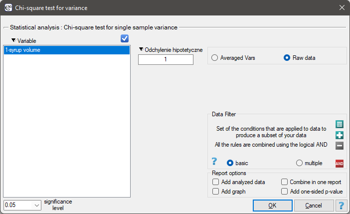
he settings window with the Chi-test for variance w can be opened in Statistics menu→Parametric tests→Chi-square test for variance.

Note

Calculations can be based on raw data or data that are averaged like: standard deviation and sample size.

EXAMPLE (dispenser.pqs file)

Before starting the production of another batch of a certain cough syrup, control measurements of the volume of syrup poured into the bottles were made. The technical documentation of the dosing device shows that the permissible variation in syrup volume measured by the standard deviation is 1ml. It should be verified that the tested device is working properly.

The distribution of the volume of syrup poured into the bottles was checked (with the Lilliefors test) obtaining a result consistent with this distribution. The analysis concerning the standard deviation can therefore be performed with the chi-square test for variance

Hypotheses:

$\begin{array}{cl} \mathcal{H}_0: & $the standard deviation of the volume of syrup$\\ &$ poured by the dosing device is 1ml,$\\ \mathcal{H}_1: & $the standard deviation of the volume of syrup$ \\ &$poured by the dosing device is other than 1ml.$ \end{array}$

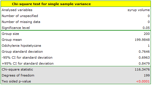
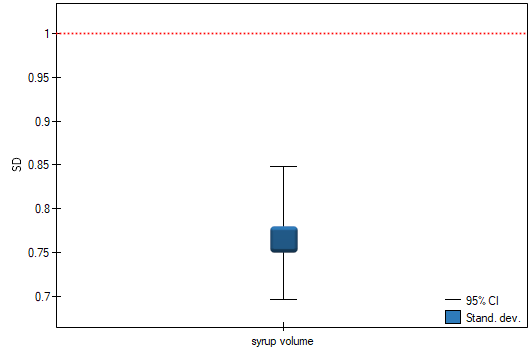
Comparing the $p<0.0001$ value of the $\chi^2$ test with the significance level $\alpha=0.05$ we find that the scatter of the dispensing device is different from 1ml. However, we can consider the performance of the device as correct because the standard deviation of the sample is 0.76, which is significantly less than the acceptable value from the technical documentation.

2022/02/09 12:56

¹⁾

Cohen J. (1988), Statistical Power Analysis for the Behavioral Sciences, Lawrence Erlbaum Associates, Hillsdale, New Jersey

PQStat - Baza Wiedzy

Narzędzia użytkownika

Narzędzia witryny

Pasek boczny

Spis treści

Parametric tests

The t-test for a single sample

The Single-Sample Chi-square Test for a Population Variance

Narzędzia strony