Spis treści

Power and sample size for test
Two independent proportions, chi-square (2x2)
- - One-way ANOVA for independent groups
  - Test for one proportion

Power and sample size for test

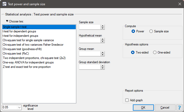
The window with the test power settings and the required sample size for this test is opened with menu Advanced Statistics→Test power and sample size→Power and sample size for test.

Power analysis is directly related to testing hypotheses, and therefore to specific statistical tests. Tests vary in their power. Some tests are stronger, others weaker. Because of this fact, if there are several tests available to solve a given statistical problem, it is better to choose the test which is more powerful. Such a test is stronger, so it will more easily reject the null hypothesis, and therefore it will be easier for us to prove the alternative hypothesis - which is, after all, the goal.

Power of statistical test is the ability of a test to detect differences, relations, correlations and any kind of dependencies which are described in alternative hypothesis. In technical language, the power of a test is called the probability of accepting an alternative hypothesis when it is in fact true.

The power of the test can be checked a priori, i.e. before collecting the data for the actual test, but often it is the reviewers of the papers or ourselves already during the analyses, i.e. a'posteriori, i.e. after collecting the actual sample, who are interested in the power of the analyses we perform. If the power of the test is low, then the results obtained may be ambiguous, if it is high - we may expect that in the future it will be difficult for other researchers to obtain different results, i.e. to undermine our results. For example, when we show using a test with a power of 80% that two groups of students are statistically significantly different from each other in terms of the number of correctly solved tasks, this means that when other researchers repeat this experiment under the same conditions as we do, they will also prove the alternative hypothesis in 80% of the random samples of the same size as ours, using the same test and assuming the same significance level.

Power of the test is determined by the formula: $\begin{displaymath} Power=1 - \beta, \end{displaymath}$

where:

$\beta$ - Type II error, which is the probability of accepting the null hypothesis when it is false.

The power of a test is directly related to the sample size $n$ - the larger the sample, the greater the power, i.e., the more students we collect to run the test, the easier it will be to argue that the detected differences between groups are not due to chance, but actually occur between populations. Hence, using the same approach, you may be interested in determining the required sample size for a given statistical test while keeping its power at a given level. In PQStat, we can calculate the power of a test by specifying the sample size, or we can calculate the sample size by specifying the test power we want to achieve. Unfortunately, both test power and sample size, in addition to being related to each other, also depend on other additional information about the collected sample that needs to be determined, these are:

The effect size $ES$ that we consider important. The larger the effect, the greater the power and the smaller the sample needed to obtain this power. For example, obtaining a difference of five correctly solved tasks will be easier to argue that the groups do in fact differ (we will have a more powerful argument) than if we tried to argue for a real advantage of one of the student groups by stating that they differ by only one correctly solved task.

To determine power or the required size, usually the effect under study must be standardized, so in many situations it is necessary to provide additional information, e.g., standard deviation, correlation coefficient, and other coefficients to standardize such an effect.

The level of statistical significance $\alpha$ (error of type I) - the greater the significance level, the greater the power. Unfortunately, the significance level is the part of the analysis over which we have only apparent influence, that is, there are few situations when it can be changed, and if a change is allowed, it involves decreasing $\alpha$ (see Multicomparison). Normally we assume that $\alpha=0.05$ .
Direction of hypothesis i.e. two-sided hypothesis (equality in null hypothesis) or one-sided hypothesis (< or > signs in null hypothesis).The one-sided hypothesis gives more power but is much less often chosen because in real life situations when applying a statistical test we rarely assume that, for example, students from the first population have no chance of beating students from the second population, but often we give equal chances to both groups at the start.

Before you can determine the power of a test, you should know how to use it, understand its hypotheses, and be able to determine the effect size, and if you have data from a study such as a pilot study, you should also perform that test.

Single-sample t-test

Before determining the power or the required sample size of the Single-sample t-test, it is worthwhile to familiarize yourself with the rules of its application.

To determine the power of the test and the required sample size, we need:

$\begin{tabular}{|c|c|} \hline \cellcolor{lightgray}\textbf{Power of the test} & \cellcolor{lightgray}\textbf{Group size} \\\hline Group size & Power of the test \\\hline \multicolumn{2}{|c|} {Hypothetical mean}\\\hline \multicolumn{2}{|c|} {Group mean}\\\hline \multicolumn{2}{|c|} {Group standard deviation}\\\hline \multicolumn{2}{|c|} {$\alpha$ significance level}\\\hline \end{tabular}$

The set effect size, in this case, is the size of the difference between the set mean of the study population and the hypothetical mean value.

The power of the test and the required sample size are calculated based on the noncentral t-test distribution.

EXAMPLE

We want to test (at the 0.05 significance level) whether the wait time for a certain delivery company to deliver a package is on average days (i.e., 72 hours).

Testing a priori - We plan to conduct a study, but have not collected data yet.

We set the test power we want to obtain at 80%.

The standard deviation that we provide should reflect the difference in delivery time that we expect to obtain in the planned study - we assume (based on the experience of the employees of this company) that it will be 1 day (24 hours).

a) What will be the required sample size when we assume that the effect size at which we would like to obtain statistical significance is 12 hours (0.5 days)?

b) What will be the required sample size when we assume that the effect size at which we would like to obtain statistical significance is 6 hours (0.25 days)?

Answer a) We know that the range from 2.5 to 3.5 days is within acceptable limits. Therefore, we use 3 days as the hypothetical mean and 2.5 days (or 3.5 days) as the test group mean.

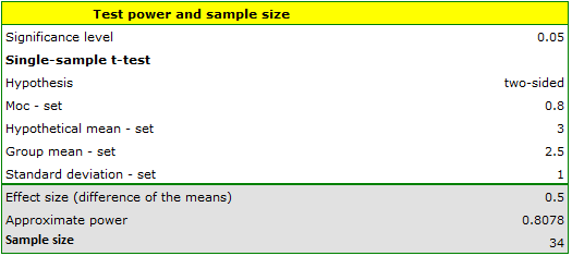
The resulting required sample size to prove that an effect exceeding 12 hours is statistically significant is 34 deliveries.

Answer b) We know that the range from 2.75 to 3.25 days is within acceptable error. Therefore, we use 3 days as the hypothetical mean and 2.75 days (or 3.25 days) as the test group mean.

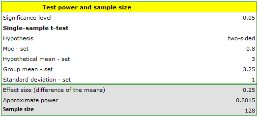
The resulting required count to prove that an effect exceeding 6 hours is statistically significant is 128 deliveries.

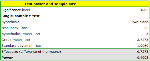
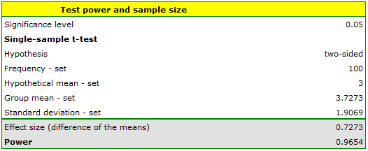
Testing a posteriori - We collected data for the study - our sample includes 22 deliveries (data in file kurier.pqs).

Based on the collected data, we determine the mean number of days to wait for delivery and the standard deviation of the group. In this case mean=3.727273, deviation=1.906925.

a) What is the power of the analysis performed?

b) What would the power look like if we increased the sample size to 100 elements while leaving the other assumptions unchanged?

Answer a) The power of the analysis performed is only 0.400302.

From this we know that many random samples with a sample size of 22 (about 60% of such samples) will not lead to confirmation of the alternative hypothesis.

Answer b) The power of our analysis will increase to 0.965364 when its sample size increases to 100 elements and the assumptions of the analysis do not change.

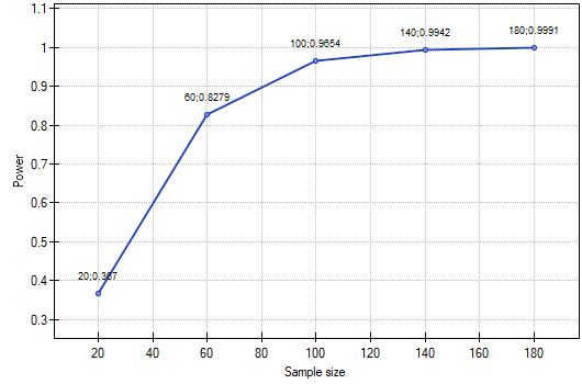
We can see how the power of the analysis will change with the sample size changing and the other assumptions unchanged in the chart.

T-test for dependent groups

Before determining the power or the required sample size of the t-test for dependent groups, it is worthwhile to familiarize yourself with the rules of its application.

To determine the power of the test and the required sample size, we need:

$\begin{tabular}{|c|c|} \hline \cellcolor{lightgray}\textbf{Power of the test} & \cellcolor{lightgray}\textbf{Group size} \\\hline Group size & Power of the test \\\hline \multicolumn{2}{|c|} {Group mean 1}\\\hline \multicolumn{2}{|c|} {Group mean 2}\\\hline \multicolumn{2}{|c|} {Standard deviation of the difference}\\ \multicolumn{2}{|c|} {(or deviations of both groups}\\ \multicolumn{2}{|c|} {and Pearson correlation coefficient)}\\\hline \multicolumn{2}{|c|} {Significance level $\alpha$}\\\hline \end{tabular}$

The set effect size, in this case, is the the difference between means that we expect to obtain in the population.

The power of the test and the required sample size are calculated based on the noncentral t-test distribution.

EXAMPLE

We want to test (at the 0.05 significance level) whether treating an eating disorder at a certain clinic produces a significant reduction in body weight after just 30 days of following a new type of diet. We consider a change in BMI of half a unit to be a significant change in body weight. How large a sample should be collected for a difference of this magnitude to be statistically significant in a t-test for dependent groups?

Because we do not have data from the pilot study, we will provide the basic data for the calculations based on the experience and estimates of the clinic staff.

We assume that the average BMI of the treated person is 35 - such a value is entered in the box for the first mean. Since a change in BMI of less than half a unit is clinically insignificant, only a decrease below 34.5 (or an increase above 35.5) will be considered significant. Thus, we report a value of 34.5 (or 35.5) as the second mean. We presume that the standard deviation of the difference (BMI before and BMI after) may be quite large, because usually the group will include people who are disciplined to follow a diet and those who still enjoy extra snacks between meals. Therefore, we set the deviation to 2.5. The power of the analysis we want to obtain is 80.

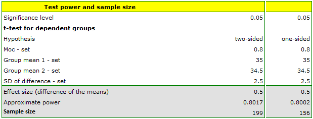
The resulting required sample size is 199 individuals when the hypothesis is two-sided (i.e., we assume that BMI may decrease or increase as a result of diet) or 156 individuals when the hypothesis is one-sided (i.e., we assume only a decrease in BMI).

If we assumed that the group would be more disciplined and the standard deviation of the difference would be 1.5 BMI units, then the sample could be slightly smaller i.e. 73 individuals for the two-sided hypothesis test and 58 individuals for the one-sided hypothesis.

T-test for independent groups

Before determining the power or the required sample size of the t-test for independent groups, it is worthwhile to familiarize yourself with the rules of its application.

To determine the power of the test and the required sample size, we need:

$\begin{tabular}{|c|c|} \hline \cellcolor{lightgray}\textbf{Power of the test} & \cellcolor{lightgray}\textbf{Group size} \\\hline Group size 1 & \multirow{2}{*}{Power of the test} \\ Group size 2 \\\hline \multicolumn{2}{|c|} {Group mean 1}\\\hline \multicolumn{2}{|c|} {Group mean 2}\\\hline \multicolumn{2}{|c|} {Common standard deviation}\\ \multicolumn{2}{|c|} {(or deviations of both groups)}\\\hline \multicolumn{2}{|c|} {Significance level $\alpha$}\\\hline \end{tabular}$

The set effect size, in this case, is the difference between means that we expect to obtain between populations.

The power of the test and the required sample size are calculated based on the noncentral t-test distribution.

EXAMPLE

We are examining men with disease X and healthy men. We want to test (at the 0.05 significance level) whether the patients differ from the healthy ones in their HDL cholesterol levels. We consider a difference of 2 mg/dl to be clinically significant. How large a sample should be collected for a difference of this magnitude to be statistically significant using t-test for independent groups?

We report 40 mg/dL as the mean HDL for ill subjects and 42 mg/dL for healthy subjects. The ratio of the sample size of both groups is 1 because we assumed equal groups. We have data from the pilot study, hence we report the standard deviation for sick (13 mg/dl) and healthy (11 mg/dl) indicating additional options . The power of the analysis we want to obtain is 80.

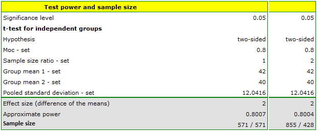
The resulting required sample size is 571 individuals when the groups are equolous (i.e., we assume due to n1/n2=1) or n1 = 855 and n2 = 428 when they are not equolous (i.e., we assume a sample size ratio of n1/n2=2)

Chi-square test for single sample variance

Before determining the power or the required sample size of the chi-square test for single sample variance, it is worthwhile to familiarize yourself with the rules of its application.

To determine the power of the test and the required sample size, we need:

$\begin{tabular}{|c|c|} \hline \cellcolor{lightgray}\textbf{Power of the test} & \cellcolor{lightgray}\textbf{Group size} \\\hline Group size & Power of the test \\\hline \multicolumn{2}{|c|} {Hypothetical standard deviation}\\\hline \multicolumn{2}{|c|} {Group standard deviation}\\\hline \multicolumn{2}{|c|} {Significance level $\alpha$}\\\hline \end{tabular}$

The set effect size, in this case, is the quotient of the standard deviation of the test population and the hypothesized deviation.

The power of the test and the required sample size is calculated based on chi-square distribution.

EXAMPLE

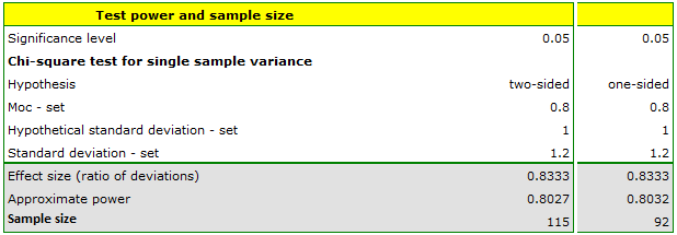
Before producing another batch of certain cough syrup, control measurements should be taken of the amount of syrup poured into the bottles. The bottles should contain 200 ml of syrup. The technical documentation of the dosing device shows that the permissible variation in syrup volume measured by the standard deviation is 1 ml. Verify (at the 0.05 significance level) that the device under test is functioning properly. Will a sample of 20 bottles be sufficient to demonstrate excessive device error, if any? A standard deviation greater than 1.2 ml is considered excessive device error.

Since we expect the standard deviation for the dispenser to be as documented we enter a value of 1 ml as a hypothetical value. We will get too big error if the deviation exceeds 1.2 ml. We enter this value in the standard deviation box for the group of bottles we are going to test.

If the sample is 20 bottles, the resulting power using the two-sided hypothesis is only 0.25, and assuming the one-sided hypothesis is only 0.34. These are low values because less than 35% random samples of will detect a device error of 0.2 ml.

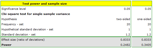
It must be recognized that 20 bottles, is too small of a group to prove a too high device standard deviation, if indeed there is one. We would like to obtain a standard power.

To obtain a power of 80% we change the program settings and calculate the required sample size, which in this case will be 115 for the two-sided hypothesis and 92 for the one-sided hypothesis.

Chi-square test of two variances Fisher-Snedecor

Before determining the power or the required sample size of the Fisher-Snedecor test, it is worthwhile to familiarize yourself with the rules of its application.

To determine the power of the test and the required sample size, we need:

$\begin{tabular}{|c|c|} \hline \cellcolor{lightgray}\textbf{Power of the test} & \cellcolor{lightgray}\textbf{Group size} \\\hline Group size 1 & \multirow{2}{*}{Power of the test} \\ Group size 2 \\\hline \multicolumn{2}{|c|} {Group 1 standard deviation}\\\hline \multicolumn{2}{|c|} {Group 2 standard deviation}\\\hline \multicolumn{2}{|c|} {Significance level $\alpha$}\\\hline \end{tabular}$

The set effect size, in this case, is the quotient of the standard deviation of populations one and two.

The power of the test and the required sample size is calculated based on the F-Snedecor distribution.

EXAMPLE

Before producing another batch of certain cough syrup, control measurements should be taken of the amount of syrup poured into the bottles. There should be 300 ml of syrup in the bottles. Two dispensing devices are used in the bottling plant. We want to test (at the 0.05 significance level) whether the distribution of syrup volume as measured by the standard deviation for the two devices is the same. A small pilot study was conducted and the standard deviation for the first device was found to be 1.32 and for the second device 1.1. If the difference is small, i.e., the quotient of the two deviations is below 1.2 (as in the pilot study), both devices will be used interchangeably; if not, the one with the smaller deviation from the mean will be chosen. How many randomly selected bottles should be measured to show that a ratio of 1.2 is statistically significant?

We enter the value of the standard deviations obtained in the pilot study and assume an 80% power of the test.

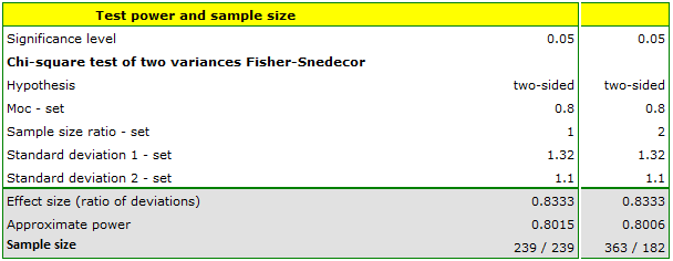
The resulting sample size for each device is n1=n2=239, assuming equal groups (i.e., ratio n1/n2=1) and n1=363 and n2=182 assuming twice the sample size for the first device (i.e., ratio n1/n2=2).

Chi-square test (goodness of fit)

Before determining the power or the required sample size of the chi-square test (goodness of fit), it is worthwhile to familiarize yourself with the rules of its application.

To determine the power of the test and the required sample size, we need¹⁾:

$\begin{tabular}{|c|c|} \hline \cellcolor{lightgray}\textbf{Power of the test} & \cellcolor{lightgray}\textbf{Group size} \\\hline Group size & \multirow{2}{*}{Power of the test} \\ Number of categories \\\hline \multicolumn{2}{|c|} {Effect size $\phi$}\\\hline \multicolumn{2}{|c|} {Significance level $\alpha$}\\\hline \end{tabular}$

The set effect size, or $\phi$ , in this case is the root of the quotient of the chi-square test statistic and the group size: $\begin{displaymath} \phi=\sqrt{\frac{\chi^2}{n}}. \end{displaymath}$ The power of the test and the required sample size are calculated based on a noncentral chi-square distribution.

Chi-square test (RxC)

Before determining the power or the required sample size of the Chi-square test RxC it is worthwhile to familiarize yourself with the rules of its application.

To determine the power of the test and the required sample size, we need²⁾³⁾:

$\begin{tabular}{|c|c|} \hline \cellcolor{lightgray}\textbf{Power of the test} & \cellcolor{lightgray}\textbf{Group size} \\\hline Group size & \multirow{3}{*}{Power of the test} \\ Number of categories (rows)\\ Number of categories (columns)\\\hline \multicolumn{2}{|c|} {Effect size $\phi$}\\\hline \multicolumn{2}{|c|} {Significance level $\alpha$}\\\hline \end{tabular}$

The set effect size, or $\phi$ , in this case is the root of the quotient of the chi-square test statistic and the group size: $\begin{displaymath} \phi=\sqrt{\frac{\chi^2}{n}}. \end{displaymath}$ The power of the test and the required sample size are calculated based on a noncentral chi-square distribution.

EXAMPLE

There are plans to conduct a large survey showing the knowledge of the Polish population about ways of fighting common viruses. The project should determine whether educational activities informing about the ineffectiveness of antibiotic therapy in viral infections were as effective in the older age group (i.e. over 50 years) as in younger adults (18-50 years). A pilot study was conducted and a random sample of 200 people was asked the question, „Do antibiotics fight viruses?” Respondents were asked the choose one of three answers: „yes”, „no” or „don't know” . The results of the pilot study were prepared for publication. The following is an excerpt from the description included in the paper:

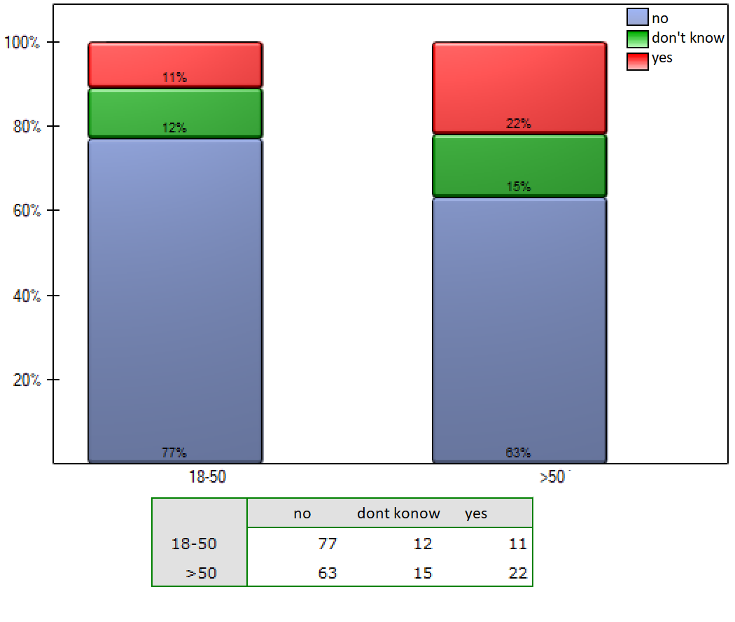
The obtained p-value in the chi-square test was statistically insignificant p=0.0672.

The paper reviewer was rightfully surprised to learn that twice as many people over the age of 50 incorrectly indicated that antibiotics fight viruses (22% vs. 11%), but this difference was not statistically significant.

As suggested by the reviewer, one should check whether the lack of statistical significance for this difference is due to the power of the test being too low, and state how large the sample should be to obtain a chi-square test power of 80% for the same percentages?

Preparing a response for the reviewer

We will determine the $\phi$ coefficient for the test (menu: Chi-square, Fisher, OR/RR→Correlation coefficients…→Phi). We obtain $\phi$ =0.1643.

Using a 200-element sample, with data placed in a table with two rows and three columns, and a given coefficient value of $\phi$ , we determine the power of the chi-square test.

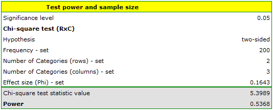
The power obtained in this analysis is low at 0.5368, which seems to confirm concerns about under-sampling.

If we get the same distribution of data for a sample with a different sample size, that means we also get the same coefficient $\phi$ . To determine the sample size that would give us an 80% power of chi-square test, we again give the coefficient $\phi$ =0.1643.

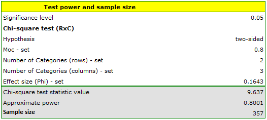
We obtain information that a sample size of 357 respondents will be needed. Since this is only a pilot study, we plan to increase the sample size to 357 respondents in the actual study.

However, we can already see that when omitting the undecided (i.e., those who chose the answer „don't know”) and redoing the analysis, significant differences can be found (chi-square, p=0.0251). In the decided group, the percentages choosing the wrong answer are more than doubled to the detriment of those aged >50 years (12.5% vs 25.9%).

Two independent proportions, chi-square (2x2)

Before determining the power or the required sample size of the chi-square (2x2) and Z test for two independent proportions It is worthwhile to familiarize yourself with the rules of their application. To determine the power of the test and the required sample size, we need⁴⁾:

$\begin{tabular}{|c|c|} \hline \cellcolor{lightgray}\textbf{Power of the test} & \cellcolor{lightgray}\textbf{Group size} \\\hline Group size & Power of the test\\\hline \multicolumn{2}{|c|} {The proportion in the first group}\\\hline \multicolumn{2}{|c|} {The proportion in the second group}\\\hline \multicolumn{2}{|c|} {Significance level $\alpha$}\\\hline \end{tabular}$

The set effect size, is the difference between the highlighted proportions.

The test value and the required sample size are calculated based on the normal distribution normal distribution.

EXAMPLE

Consider a study evaluating the effectiveness of aspirin in reducing mortality from myocardial infarction. Previous studies indicate that the rate of death from myocardial infarction is 0.015 for nonusers and 0.001 for aspirin users. The researchers want to determine the minimum sample size required to detect an absolute difference | 0.001-0.015 | = 0.014 at 80% power using a two-sided test with a significance level of 5%.

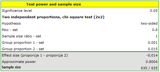
Assuming the groups are equal, 635 people need to be picked for each group.}

One-way ANOVA for independent groups

Before determining the power or the required sample size of the One-way ANOVA for independent groups It is worthwhile to familiarize yourself with the rules of its application.

To determine the power of the test and the required sample size, we need:

$\begin{tabular}{|c|c|} \hline \cellcolor{lightgray}\textbf{Power of the test} & \cellcolor{lightgray}\textbf{Group size} \\\hline Group size & Power of the test \\\hline \multicolumn{2}{|c|} {Group 1 mean}\\\hline \multicolumn{2}{|c|} {Group 2 mean}\\\hline \multicolumn{2}{|c|} {Group 3 mean}\\\hline \multicolumn{2}{|c|} {Group 4 mean}\\\hline \multicolumn{2}{|c|} {Group 1 standard deviation}\\\hline \multicolumn{2}{|c|} {Group 2 standard deviation}\\\hline \multicolumn{2}{|c|} {Group 3 standard deviation}\\\hline \multicolumn{2}{|c|} {Group 4 standard deviation}\\\hline \multicolumn{2}{|c|} {Significance level $\alpha$}\\\hline \end{tabular}$

The set effect size, in this case, is the RMSSE, which is the standardized measure used in ANOVA to describe the overall level of effect in the population.

The power of the test and the requiredy sample size are calculated based on the non-central F-Snedecor distribution.

EXAMPLE

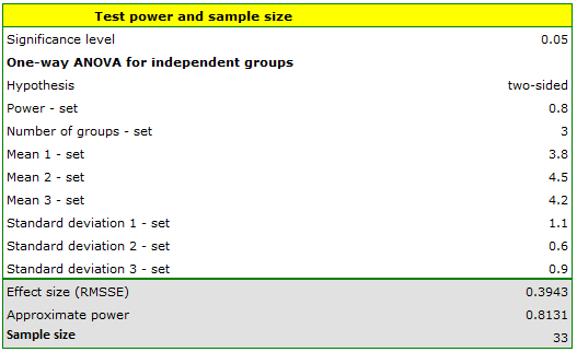
The FVC parameter was studied for patients with heart defects (heart defect A, heart defect B and heart defect C). We want to find out (at a significance level of 0.05) whether the patients differ in the values of this parameter. To test this, a pilot study was first conducted. Based on the results of this study, the predicted effect sizes were determined, i.e:

- for heart defect A: mean = 3.8, standard deviation = 1.1,

- for heart defect B: mean = 4.5, standard deviation = 0.6,

- for heart defect C: mean = 4.2, standard deviation = 0.9.

How many people should be gathered if the quantities remain the same to prove that there are statistically significant differences?

We enter values for means and standard deviations. The resulting sample size for each of the study groups is 33, assuming an 80% power of the test.

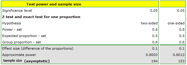
Test for one proportion

Before determining the power or the required sample size of the test for one proportion it is worthwhile to familiarize yourself with the rules of its application.

To determine the power of the test and the required sample size, we need:

$\begin{tabular}{|c|c|} \hline \cellcolor{lightgray}\textbf{Power of the test} & \cellcolor{lightgray}\textbf{Group size} \\\hline Group size & Power of the test \\\hline \multicolumn{2}{|c|} {Expected proportion}\\\hline \multicolumn{2}{|c|} {Group proportion}\\\hline \multicolumn{2}{|c|} {Significance level $\alpha$}\\\hline \end{tabular}$

The set effect size, in this case, is the amount of difference between the set proportion in the study population and the hypothetical expected proportion.

The power of the test and the required sample size are calculated based on the normal distribution when using the asymptotic test or the binomial distribution when using the exact test.

EXAMPLE

10 randomly selected families with children under the age of 10 and residing in Poznań were asked about the plans for their children's education. Of these, 6 families planned to educate their children at university. At a significance level of 0.05 and a test power of 0.8, how large a sample would we need to collect to conclude that more than 50% of the families in Poznań with children under the age of 10 are already planning for their children to attend university in the future?

We enter 0.5 as the expected proportion and 0.6 as the group proportion. The resulting sample size is 194 families-when the hypothesis being tested is two-sided or 153 families-when the hypothesis is one-sided.

¹⁾

Cohen, J. (1988), Statistical Power Analysis for the Behavioral Sciences, Lawrence Erlbaum Associates, Hillsdale, New Jersey

²⁾

Cohen J. (1988), Statistical Power Analysis for the Behavioral Sciences, Lawrence Erlbaum Associates, Hillsdale, New Jersey

³⁾

Oyeyemi G.M. , Adewara A.A., Adebola F.B. and Salau S.I. (2010), On the Estimation of Power and Sample Size in Test of Independence, Asian Journal of Mathematics and Statistics, 3(3): 139-146

⁴⁾

Chow S.C., Shao J., and Wang H. (2008), Sample Size Calculations in Clinical Research, Second Edition. Chapman and Hall/CRC. Boca Raton, Florida.

PQStat - Baza Wiedzy

Pasek boczny

Spis treści

Power and sample size for test

Single-sample t-test

T-test for dependent groups

T-test for independent groups

Chi-square test for single sample variance

Chi-square test of two variances Fisher-Snedecor

Chi-square test (goodness of fit)

Chi-square test (RxC)

Two independent proportions, chi-square (2x2)

One-way ANOVA for independent groups

Test for one proportion

PQStat - Baza Wiedzy

Narzędzia użytkownika

Narzędzia witryny

Pasek boczny

Spis treści

Power and sample size for test

Single-sample t-test

T-test for dependent groups

T-test for independent groups

Chi-square test for single sample variance

Chi-square test of two variances Fisher-Snedecor

Chi-square test (goodness of fit)

Chi-square test (RxC)

Two independent proportions, chi-square (2x2)

One-way ANOVA for independent groups

Test for one proportion

Narzędzia strony