Narzędzia użytkownika
Narzędzia witryny
Pasek boczny
en:statpqpl:porown2grpl:nparpl:z_nzalrpl
The Z test for 2 independent proportions
The  test for 2 independent proportions is used in the similar situations as the Chi-square test (2x2). It means, when there are 2 independent samples with the total size of
  and
and  , with the 2 possible results to gain (one of the results is distinguished with the size of
  - in the first sample and
  - in the second one). For these samples it is also possible to calculate the distinguished proportions
  and
and  . This test is used to verify the hypothesis informing us that the distinguished proportions
  and
and  in populations, from which the samples were drawn, are equal.
Basic assumptions:
- measurement on a nominal scale - any order is not taken into account,
- large sample sizes.
Hypotheses:

where:
, fraction for the first and the second population.
The test statistic is defined by:

where:
 .
.
The test statistic modified by the continuity correction is defined by:

The Statistic with and without the continuity correction asymptotically (for the large sample sizes) has the normal distribution.
The p-value, designated on the basis of the test statistic, is compared with the significance level  :
:

Apart from the difference between proportions, the program calculates the value of the NNT.
NNT (number needed to treat) – indicator used in medicine to define the number of patients which have to be treated for a certain time in order to cure one person.
NNT is calculated from the formula:

and is quoted when the difference  is positive.
NNH (number needed to harm) – an indicator used in medicine, denotes the number of patients whose exposure to a risk over a specified period of time, results in harm to one person who would not otherwise be harmed. NNH is calculated in the same way as NNT, but is quoted when the difference is negative.
Confidence interval – The narrower the confidence interval, the more precise the estimate. If the confidence interval includes 0 for the difference in proportions and  for the NNT and/or NNH, then there is an indication to treat the result as statistically insignificant
Note
From PQStat version 1.3.0, the confidence intervals for the difference between two independent proportions are estimated on the basis of the Newcombe-Wilson method. In the previous versions it was estimated on the basis of the Wald method.
The justification of the change is as follows:
Confidence intervals based on the classical Wald method are suitable for large sample sizes and for the difference between proportions far from 0 or 1. For small samples and for the difference between proportions close to those extreme values, the Wald method can lead to unreliable results (Newcombe 19981), Miettinen 19852), Beal 19873), Wallenstein 19974)). A comparison and analysis of many methods which can be used instead of the simple Wald method can be found in Newcombe's study (1998)5). The suggested method, suitable also for extreme values of proportions, is the method first published by Wilson (1927)6), extended to the intervals for the difference between two independent proportions.
Note
The confidence interval for NNT and/or NNH is calculated as the inverse of the interval for the proportion, according to the method proposed by Altman (Altman (1998)7)).
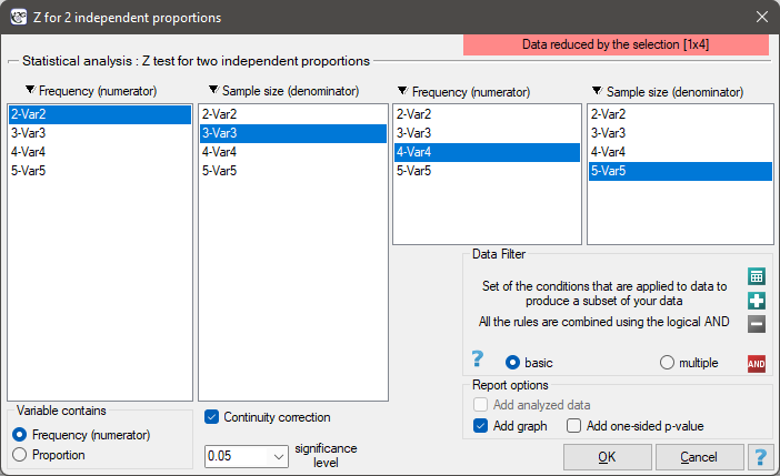
The settings window with the Z test for 2 proportions can be opened in Statistics menu → NonParametric tests → Z for 2 independent proportions.
EXAMPLE cont. (sex-exam.pqs file)
You know that  out of all the women in the sample who passed the exam and
  out of all the men in the sample who passed the exam.
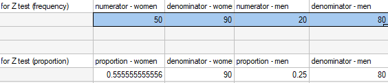
This data can be written in two ways – as a numerator and a denominator for each sample, or as a proportion and a denominator for each sample:
out of all the men in the sample who passed the exam.
This data can be written in two ways – as a numerator and a denominator for each sample, or as a proportion and a denominator for each sample:
Hypotheses:

Note
It is necessary to select the appropriate area (data without headings) before the analysis begins, because usually there are more information in a datasheet. You should also select the option indicating the content of the variable (frequency (numerator) or proportion).
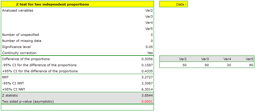
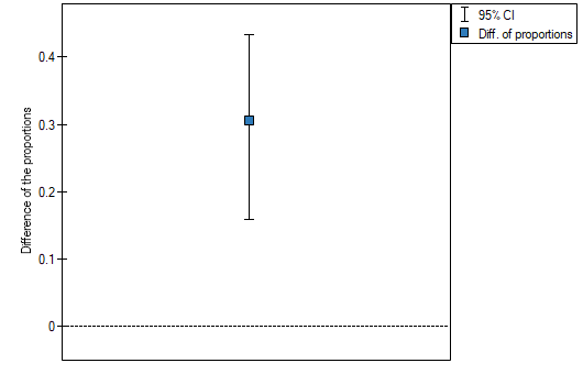
The difference between proportions distinguished in the sample is 30.56%, a 95% and the confidence interval for it  does not contain 0.
Based on the test without the continuity correction as well as on the test with the continuity correction ( p-value < 0.0001), on the significance level =0.05, the alternative hypothesis can be accepted (similarly to the Fisher exact test, its the mid-p corrections, the  test and the test with the Yate's correction). So, the proportion of men, who passed the exam is different than the proportion of women, who passed the exam in the analysed population. Significantly, the exam was passed more often by women (
 out of all the women in the sample who passed the exam) than by men ( out of all the men in the sample who passed the exam).
EXAMPLE
Let us assume that the mortality rate of a disease is 100\% without treatment and that therapy lowers the mortality rate to 50% – that is the result of 20 years of study. We want to know how many people have to be treated to prevent 1 death in 20 years. To answer that question, two samples of 100 people were taken from the population of the diseased. In the sample without treatment there are 100 patients of whom we know they will all die without the therapy. In the sample with therapy we also have 100 patients of whom 50 will survive. \small{

We will calculate the NNT.
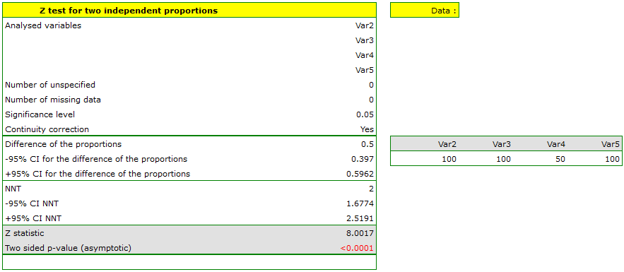
The difference between proportions is statistically significant ( ) but we are interested in the NNT – its value is 2, so the treatment of 2 patients for 20 years will prevent 1 death. The calculated confidence interval value of 95\% should be rounded off to a whole number, wherefore the NNT is 2 to 3 patients.
EXAMPLE
The value of the certain proportion difference in the study comparing the effectiveness of drug 1 vs drug 2 was: difference (95%CI)=-0.08 (-0.27 do 0.11). This negative proportion difference suggests that drug 1 was less effective than drug 2, so its use put patients at risk. Because the proportion difference is negative, the determined inverse is called the NNH, and because the confidence interval contains infinity NNH(95\%CI)= 2.5 (NNH 3.7 to ∞ to NNT 9.1) and goes from NNH to NNT, we should conclude that the result obtained is not statistically significant (Altman (1998)8)).
1)
, 5)
Newcombe R.G. (1998), Interval Estimation for the Difference Between Independent Proportions: Comparison of Eleven Methods. Statistics in Medicine 17: 873-890
2)
Miettinen O.S. and Nurminen M. (1985), Comparative analysis of two rates. Statistics in Medicine 4: 213-226
3)
Beal S.L. (1987), Asymptotic confidence intervals for the difference between two binomial parameters for use with small samples. Biometrics 43: 941-950
4)
Wallenstein S. (1997), A non-iterative accurate asymptotic confidence interval for the difference between two Proportions. Statistics in Medicine 16: 1329-1336
6)
Wilson E.B. (1927), Probable Inference, the Law of Succession, and Statistical Inference. Journal of the American Statistical Association: 22(158):209-212
en/statpqpl/porown2grpl/nparpl/z_nzalrpl.txt · ostatnio zmienione: 2022/02/12 15:45 przez admin
Narzędzia strony
Wszystkie treści w tym wiki, którym nie przyporządkowano licencji, podlegają licencji: CC Attribution-Noncommercial-Share Alike 4.0 International
