PQStat - Baza Wiedzy

Spis treści

Parametric tests

Parametric tests

The linear correlation coefficients

The Pearson product-moment correlation coefficient $r_p$ called also the Pearson's linear correlation coefficient (Pearson (1896,1900)) is used to decribe the strength of linear relations between 2 features. It may be calculated on an interval scale as long as there are no measurement outliers and the distribution of residuals or the distribution of the analyed features is a normal one.

$\begin{displaymath} r_p=\frac{\sum_{i=1}^n(x_i-\overline{x})(y_i-\overline{y})}{\sqrt{\sum_{i=1}^n(x_i-\overline{x})^2}\sqrt{\sum_{i=1}^n(y_i-\overline{y})^2}}, \end{displaymath}$

where:

$x_i, y_i$ - the following values of the feature $X$ and $Y$ ,

$\overline{x}, \overline{y}$ - means values of features: $X$ and $Y$ ,

$n$ - sample size.

Note

$R_p$ – the Pearson product-moment correlation coefficient in a population;

$r_p$ – the Pearson product-moment correlation coefficient in a sample.

The value of $r_p\in<-1; 1>$ , and it should be interpreted the following way:

$r_p\approx1$ means a strong positive linear correlation – measurement points are closed to a straight line and when the independent variable increases, the dependent variable increases too;
$r_p\approx-1$ means a strong negative linear correlation – measurement points are closed to a straight line, but when the independent variable increases, the dependent variable decreases;
if the correlation coefficient is equal to the value or very closed to zero, there is no linear dependence between the analysed features (but there might exist another relation - a not linear one).

Graphic interpretation of $r_p$ .

$\begin{pspicture}(0,-.8)(12.5,2.5) \psline{->}(.5,0)(.5,2) \psline{->}(.5,0)(2.5,0) \rput(.8,1){*} \rput(1.7,.9){*} \rput(1,.7){*} \rput(1.3,1.6){*} \rput(1.5,1){*} \rput(1.1,.4){*} \rput(2.1,1){*} \rput(1.9,1.8){*} \rput(.2,2){$y$} \rput(2.5,-.2){$x$} \rput(1.5,-.7){$r_p\approx0$} \psline{->}(4.5,0)(4.5,2) \psline{->}(4.5,0)(6.5,0) \psline{-}(4.7,.5)(6.3,1.8) \rput(4.8,.7){*} \rput(5.3,1){*} \rput(5,.4){*} \rput(6,1.7){*} \rput(5.7,1.2){*} \rput(4.2,2){$y$} \rput(6.5,-.2){$x$} \rput(5.5,-.7){$r_p\approx1$} \psline{->}(8.5,0)(8.5,2) \psline{->}(8.5,0)(10.5,0) \psline{-}(8.7,1.8)(10.3,.2) \rput(9.6,.9){*} \rput(8.9,1.4){*} \rput(9.7,1.2){*} \rput(10.1,.2){*} \rput(9.9,.4){*} \rput(8.2,2){$y$} \rput(10.5,-.2){$x$} \rput(9.5,-.7){$r_p\approx-1$} \end{pspicture}$

If one out of the 2 analysed features is constant (it does not matter if the other feature is changed), the features are not dependent from each other. In that situation $r_p$ can not be calculated.

Note

You are not allowed to calculate the correlation coefficient if: there are outliers in a sample (they may make that the value and the sign of the coefficient would be completely wrong), if the sample is clearly heterogeneous, or if the analysed relation takes obviously the other shape than linear.

The coefficient of determination: $r_p^2$ – reflects the percentage of a dependent variable a variability which is explained by variability of an independent variable.

A created model shows a linear relationship: $\begin{displaymath} y=\beta x+\alpha. \end{displaymath}$ $\beta$ and $\alpha$ coefficients of linear regression equation can be calculated using formulas: $\begin{displaymath} \displaystyle{\beta=\frac{\sum_{i=1}^n(x_i-\overline{x})(y_i-\overline{y})}{\sum_{i=1}^n(x_i-\overline{x})^2}}, \qquad \alpha=\overline{y}-\beta\overline{x}. \end{displaymath}$

EXAMPLE cont. (age-height.pqs file)

2022/02/09 12:56

The Pearson correlation coefficient significance

The test of significance for Pearson product-moment correlation coefficient is used to verify the hypothesis determining the lack of linear correlation between an analysed features of a population and it is based on the Pearson's linear correlation coefficient calculated for the sample. The closer to 0 the value of coefficient $r_p$ is, the weaker dependence joins the analysed features.

Basic assumptions:

measurement on the interval scale,
normality of distribution of residuals or an analysed features in a population.

Hypotheses:

$\begin{array}{cl} \mathcal{H}_0: & R_p = 0, \\ \mathcal{H}_1: & R_p \ne 0. \end{array}$

The test statistic is defined by: $\begin{displaymath} t=\frac{r_p}{SE}, \end{displaymath}$

where $\displaystyle SE=\sqrt{\frac{1-r_p^2}{n-2}}$ .

The value of the test statistic can not be calculated when $r_p=1$ or $r_p=-1$ or when $n<3$ .

The test statistic has the t-Student distribution with $n-2$ degrees of freedom.

The p-value, designated on the basis of the test statistic, is compared with the significance level $\alpha$ :

$\begin{array}{ccl} $ if $ p \le \alpha & \Longrightarrow & $ reject $ \mathcal{H}_0 $ and accept $ \mathcal{H}_1, \\ $ if $ p > \alpha & \Longrightarrow & $ there is no reason to reject $ \mathcal{H}_0. \\ \end{array}$

EXAMPLE cont. (age-height.pqs file)

2022/02/09 12:56

The slope coefficient significance

The test of significance for the coefficient of linear regression equation

This test is used to verify the hypothesis determining the lack of a linear dependence between an analysed features and is based on the slope coefficient (also called an effect), calculated for the sample. The closer to 0 the value of $\beta$ coefficient is, the weaker dependence presents the fitted line.

Basic assumptions:

measurement on the interval scale,
normality of distribution of residuals or an analysed features in a population.

Hypotheses:

$\begin{array}{cl} \mathcal{H}_0: & \beta = 0, \\ \mathcal{H}_1: & \beta \ne 0. \end{array}$

The test statistic is defined by:

$\begin{displaymath} t=\frac{\beta}{SE} \end{displaymath}$

where:

$\displaystyle SE=\frac{s_{yx}}{sd_x\sqrt{n-1}}$ ,

$s_{yx}=sd_y \sqrt{\frac{n-1}{n-2}(1-r^2)}$ ,

$sd_x, sd_y$ – standard deviation of the value of features: $X$ and $Y$ .

The value of the test statistic can not be calculated when $r_p=1$ or $r_p=-1$ or when $n<3$ .

The test statistic has the t-Student distribution with $n-2$ degrees of freedom.

The p-value, designated on the basis of the test statistic, is compared with the significance level $\alpha$ :

$\begin{array}{ccl} $ if $ p \le \alpha & \Longrightarrow & $ reject $ \mathcal{H}_0 $ and accept $ \mathcal{H}_1, \\ $ if $ p > \alpha & \Longrightarrow & $ there is no reason to reject $ \mathcal{H}_0. \\ \end{array}$

Prediction is used to predict the value of a one variable (mainly a dependent variable $y_0$ ) on the basis of a value of an another variable (mainly an independent variable $x_0$ ). The accuracies of a calculated value are defined by prediction intervals calculated for it.

Interpolation is used to predict the value of a variable, which occurs inside the area for which the regression model was done. Interpolation is mainly a safe procedure - it is assumed only the continuity of the function of analysed variables.
Extrapolation is used to predict the value of variable, which occurs outside the area for which the regression model was done. As opposed to interpolation, extrapolation is often risky and is performed only not far away from the area, where the regression model was created. Similarly to the interpolation, it is assumed the continuity of the function of analysed variables.

Analysis of model residuals - explanation in the Multiple Linear Regression module.

The settings window with the Pearson's linear correlation can be opened in Statistics menu→Parametric tests→linear correlation (r-Pearson) or in ''Wizard''.

EXAMPLE (age-height.pqs file)

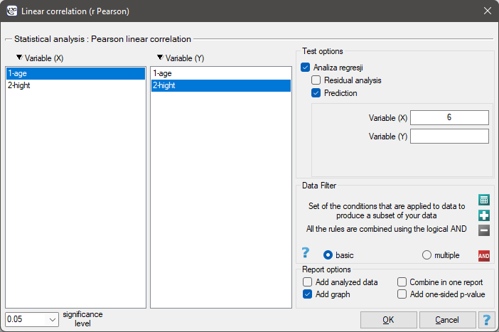
Among some students of a ballet school, the dependence between age and height was analysed. The sample consists of 16 children and the following results of these features (related to the children) were written down:

(age, height): (5, 128) (5, 129) (5, 135) (6, 132) (6, 137) (6, 140) (7, 148) (7, 150) (8, 135) (8, 142) (8, 151) (9, 138) (9, 153) (10, 159) (10, 160) (10, 162).}

Hypotheses:

$\begin{array}{cl} \mathcal{H}_0: & $there is no linear dependence between age and height$\\ &$for the population of children who attend to the analysed school,$\\ \mathcal{H}_1: & $there is a linear dependence between age and height$\\ &$for the population of children who attend to the analysed school.$ \end{array}$

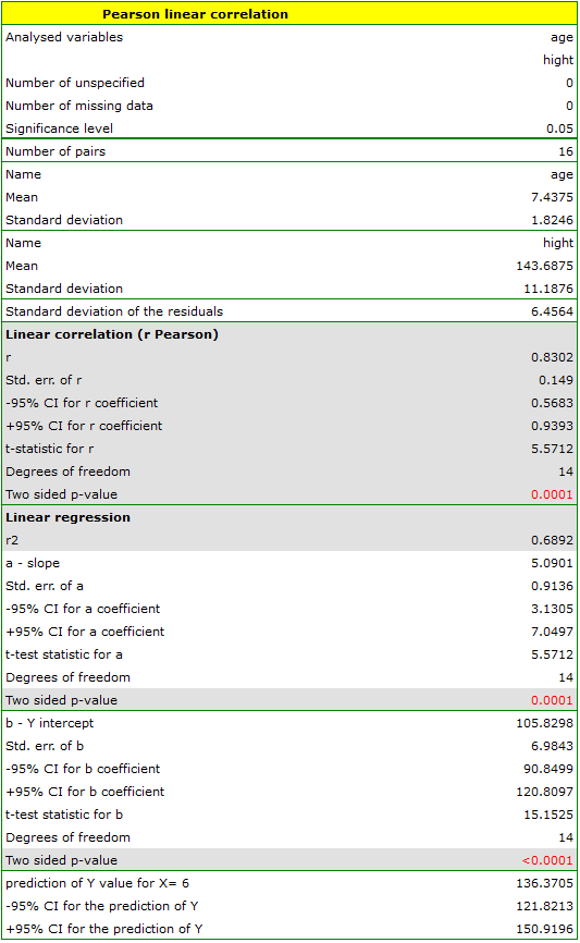
Comparing the $p$ value < 0.0001 with the significance level $\alpha=0.05$ , we draw the conclusion, that there is a linear dependence between age and height in the population of children attening to the analysed school. This dependence is directly proportional, it means that the children grow up as they are getting older.

The Pearson product-moment correlation coefficient, so the strength of the linear relation between age and height counts to $r_p$ =0.83. Coefficient of determination $r_p^2=0.69$ means that about 69\% variability of height is explained by the changing of age.

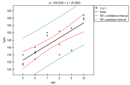
From the regression equation: $\begin{displaymath} height=5.09\cdot age +105.83 \end{displaymath}$ it is possible to calculate the predicted value for a child, for example: in the age of 6. The predicted height of such child is 136.37cm.

2022/02/09 12:56

Comparison of correlation coefficients

The test for checking the equality of the Pearson product-moment correlation coefficients, which come from 2 independent populations

This test is used to verify the hypothesis determining the equality of 2 Pearson's linear correlation coefficients ( $R_{p_1}$ , $R_{p_2})$ .

Basic assumptions:

$r_{p_1}$ and $r_{p_2}$ come from 2 samples which are chosen randomly from independent populations,
$r_{p_1}$ and $r_{p_2}$ describe the strength of dependence of the same features: $X$ and $Y$ ,
sizes of both samples ( $n_1$ and $n_2$ ) are known.

Hypotheses:

$\begin{array}{cl} \mathcal{H}_0: & R_{p_1} = R_{p_2}, \\ \mathcal{H}_1: & R_{p_1} \ne R_{p_2}. \end{array}$

The test statistic is defined by:

$\begin{displaymath} t=\frac{z_{r_{p_1}}-z_{r_{p_2}}}{\sqrt{\frac{1}{n_1-3}+\frac{1}{n_2-3}}}, \end{displaymath}$

where:

$\displaystyle z_{r_{p_1}}=\frac{1}{2}\ln\left(\frac{1+r_{p_1}}{1-r_{p_1}}\right)$ ,

$\displaystyle z_{r_{p_2}}=\frac{1}{2}\ln\left(\frac{1+r_{p_2}}{1-r_{p_2}}\right)$ .

The test statistic has the t-Student distribution with $n_1+n_2-4$ degrees of freedom.

The p-value, designated on the basis of the test statistic, is compared with the significance level $\alpha$ :

$\begin{array}{ccl} $ if $ p \le \alpha & \Longrightarrow & $ reject $ \mathcal{H}_0 $ and accept $ \mathcal{H}_1, \\ $ if $ p > \alpha & \Longrightarrow & $ there is no reason to reject $ \mathcal{H}_0. \\ \end{array}$

Note

A comparison of the slope coefficients of the regression lines can be made in a similar way. </WRAP>

2022/02/09 12:56

Comparison of the slope of regression lines

The test for checking the equality of the coefficients of linear regression equation, which come from 2 independent populations

This test is used to verify the hypothesis determining the equality of 2 coefficients of the linear regression equation $\beta_1$ and $\beta_2$ in analysed populations.

Basic assumptions:

$\beta_1$ and $\beta_2$ come from 2 samples which are chosen randomly from independent populations,
$\beta_1$ and $\beta_2$ describe the strength of dependence of the same features: $X$ and $Y$ ,
both sample sizes ( $n_1$ and $n_2$ ) are known,
standard deviations for the values of both features in both samples ( $sd_{x_1}, sd_{y_1}$ and $sd_{x_2}, sd_{y_2}$ ) are known,
the Pearson product-moment correlation coefficients of both samples ( $r_{p_1}$ and $r_{p_2}$ ) are known.

Hypotheses:

$\begin{array}{cl} \mathcal{H}_0: & \beta_1 = \beta_2, \\ \mathcal{H}_1: & \beta_1 \ne \beta_2. \end{array}$

The test statistic is defined by:

$\begin{displaymath} t=\frac{\beta_1 -\beta_2}{\sqrt{\frac{s_{yx_1}^2}{sd_{x_1}^2(n_1-1)}+\frac{s_{yx_2}^2}{sd_{x_1}^2(n_2-1)}}}, \end{displaymath}$

where:

$\displaystyle s_{yx_1}=sd_{y_1}\sqrt{\frac{n_1-1}{n_1-2}(1-r_{p_1}^2)}$ ,

$\displaystyle s_{yx_2}=sd_{y_2}\sqrt{\frac{n_2-1}{n_2-2}(1-r_{p_2}^2)}$ .

The test statistic has the t-Student distribution with $n_1+n_2-4$ degrees of freedom.

The p-value, designated on the basis of the test statistic, is compared with the significance level $\alpha$ :

$\begin{array}{ccl} $ if $ p \le \alpha & \Longrightarrow & $ reject $ \mathcal{H}_0 $ and accept $ \mathcal{H}_1, \\ $ if $ p > \alpha & \Longrightarrow & $ there is no reason to reject $ \mathcal{H}_0. \\ \end{array}$

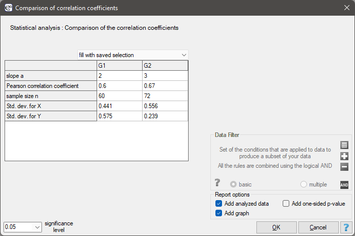
The settings window with the comparison of correlation coefficients can be opened in Statistics menu → Parametric tests → Comparison of correlation coefficients.

2022/02/09 12:56

PQStat - Baza Wiedzy

Narzędzia użytkownika

Narzędzia witryny

Pasek boczny

Spis treści

Parametric tests

The linear correlation coefficients

The Pearson correlation coefficient significance

The slope coefficient significance

Comparison of correlation coefficients

Comparison of the slope of regression lines

Narzędzia strony