PQStat - Baza Wiedzy

The ROC Curve

The diagnostic test is used for differentiating objects with a given feature (marked as (+), e.g. ill people) from objects without the feature (marked as (–), e.g. healthy people). For the diagnostic test to be considered valuable, it should yield a relatively small number of wrong classifications. If the test is based on a dichotomous variable then the proper tool for the evaluation of the quality of the test is the analysis of a $2\times2$ contingency table of true positive (TP), true negative (TN), false positive (FP), and false negative (FN) values. Most frequently, though, diagnostic tests are based on continuous variables or ordered categorical variables. In such a situation the proper means of evaluating the capability of the test for differentiating (+) and (–) are ROC (Receiver Operating Characteristic) curves.

It is frequently observed that the greater the value of the diagnostic variable, the greater the odds of occurrence of the studied phenomenon, or the other way round: the smaller the value of the diagnostic variable, the smaller the odds of occurrence of the studied phenomenon. Then, with the use of ROC curves, the choice of the optimum cut-off is made, i.e. the choice of a certain value of the diagnostic variable which best separates the studied statistical population into two groups: (+) in which the given phenomenon occurs and (–) in which the given phenomenon does not occur.

When, on the basis of the studies of the same objects, two or more ROC curves are constructed, one can compare the curves with regard to the quality of classification.

Let us assume that we have at our disposal a sample of $n$ elements, in which each object has one of the $k$ values of the diagnostic variable. Each of the received values of the diagnostic variable $x_1, x_2, ...x_k$ becomes the cut-off $x_{cat}$ .

If the diagnostic variable is:

stimulant (the growth of its value makes the odds of occurrence of the studied phenomenon greater), then values greater than or equal to the cut-off ( $x_i>=x_{cat}$ ) are classified in group (+);
destimulant (the growth of its value makes the odds of occurrence of the studied phenomenon smaller), then values smaller than or equal to the cut-off ( $x_i>=x_{cat}$ ) are classified in group (+);

For each of the $k$ cut-offs we define true positive (TP), true negative (TN), false positive (FP), and false negative (FN) values.

$\begin{tabular}{|c|c||c|c|} \hline \multicolumn{2}{|c||}{stimulant}& \multicolumn{2}{|c|}{Reality} \\\cline{3-4} \multicolumn{2}{|c||}{ }&\textbf{(+)}&\textbf{(--)}\\\hline \hline \multirow{2}{*}{diagnostic variable} &$x_i>=x_{cat}$ \textbf{(+)} & TP & FP \\\cline{3-4} &$x_i<x_{cat}$ \textbf{(--)}& FN &TN\\\hline \end{tabular}$

$\begin{tabular}{|c|c||c|c|} \hline \multicolumn{2}{|c||}{destimulant}& \multicolumn{2}{|c|}{Reality} \\\cline{3-4} \multicolumn{2}{|c||}{ }&\textbf{(+)}&\textbf{(--)}\\\hline \hline \multirow{2}{*}{diagnostic variable} &$x_i<=x_{cat}$ \textbf{(+)} & TP & FP \\\cline{3-4} &$x_i>x_{cat}$ \textbf{(--)}& FN &TN\\\hline \end{tabular}$

On the basis of those values each cut-off $x_{cat}$ can be further described by means of sensitivity and specificity, positive predictive values(PPV), negative predictive values (NPV), positive result likelihood ratio (LR+), negative result likelihood ratio (LR-), and accuracy (Acc).

Note

The PQStat program computes the prevalence coefficient on the basis of the sample. The computed prevalence coefficient will reflect the occurrence of the studied phenomenon (illness) in the population in the case of screening of a large sample representing the population. If only people with suspected illness are directed to medical examinations, then the computed prevalence coefficient for them can be much higher than the prevalence coefficient for the population.

Because both the positive and negative predictive value depend on the prevalence coefficient, when the coefficient for the population is known a priori, we can use it to compute, for each cut-off $x_{cat}$ , corrected predictive values according to Bayes's formulas:

$\begin{displaymath} PPV_{revised}=\frac{\textrm{Sensitivity}\cdot P_{a priori}}{\textrm{Sensitivity}\cdot P_{a priori} + (1-\textrm{Specificity})\cdot (1-P_{a priori})} \end{displaymath}$

$\begin{displaymath} NPV_{revised}=\frac{\textrm{Specificity}\cdot (1-P_{a priori})}{\textrm{Specificity}\cdot (1-P_{a priori}) + (1-\textrm{Sensitivity})\cdot P_{a priori}} \end{displaymath}$

where:

$P_{a priori}$ - the prevalence coefficient put in by the user, the so-called pre-test probability of disease

$\begin{tabular}{|c||c|c|c|c|c|c|c||c|c|} \hline \textbf{$x_{cat}$} & \textbf{sensitivity} & \textbf{specificity} & $\textbf{PPV}$ & $\textbf{NPV}$ & $\textbf{LR}_+$ & $\textbf{LR}_-$ & $\textbf{Acc}$ &$\textbf{PPV}_{rev}$ & $\textbf{NPV}_{rev}$\\\hline\hline $x_1$ & sensitivity$_1$ & specificity$_1$ & $PPV_1$ & $NPV_1$ & $LR_{+1}$ & $LR_{-1}$ & $Acc_1$ & $PPV_{rev1}$ & $NPV_{rev1}$\\\hline $x_2$ & sensitivity$_2$ & specificity$_2$ & $PPV_2$ & $NPV_2$ & $LR_{+2}$ & $LR_{-2}$ & $Acc_2$ & $PPV_{rev2}$ & $NPV_{rev2}$\\\hline \vdots & \vdots & \vdots & \vdots & \vdots & \vdots & \vdots & \vdots & \vdots & \vdots\\\hline $x_k$ & sensitivity$_k$ & specificity$_k$ & $PPV_k$ & $NPV_k$ & $LR_{+k}$ & $LR_{-k}$ & $Acc_k$ & $PPV_{revk}$ & $NPV_{revk}$\\\hline \end{tabular}$

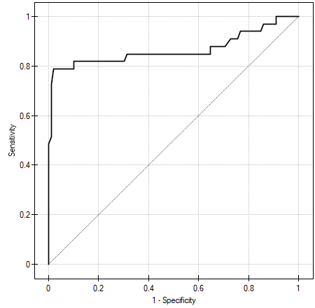
The ROC curve is created on the basis of the calculated values of sensitivity and specificity. On the abscissa axis the $x$ =1-specificity is placed, and on the ordinate axis $y$ =sensitivity. The points obtained in that manner are linked. The constructed curve, especially the area under the curve, presents the classification quality of the analyzed diagnostic variable. When the ROC curve coincides with the diagonal $y=x$ , then the decision made on the basis of the diagnostic variable is as good as the random distribution of studied objects into group (+) and group (–).

AUC (area under curve) – the size of the area under the ROC curve falls within $<0; 1>$ . The greater the field the more exact the classification of the objects in group (+) and group (–) on the basis of the analyzed diagnostic variable. Therefore, that diagnostic variable can be even more useful as a classifier. The area $AUC$ , error $SE_{AUC}$ and confidence interval for AUC are calculated on the basis of:

nonparametric DeLong method (DeLong E.R. et al. 1988¹⁾, Hanley J.A. i Hajian-Tilaki K.O. 1997²⁾) - recommended,
nonparametric Hanley-McNeil method (Hanley J.A. i McNeil M.D. 1982³⁾),
Hanley-McNeil method which presumes double negative exponential distribution (Hanley J.A. i McNeil M.D. 1982⁴⁾) - computed only when groups (+) and (–) are equinumerous.

For the classification to be better than random distribution of objects into to classes, the area under the ROC curve should be significantly larger than the area under the line $y=x$ , i.e. than 0.5.

Hypotheses:

$\begin{array}{cl} \mathcal{H}_0: & AUC=0.5, \\ \mathcal{H}_1: & AUC\neq 0.5. \end{array}$

The test statistics has the form presented below:

$\begin{displaymath} Z=\frac{AUC-0.5}{SE_{0.5}}, \end{displaymath}$

where:

$SE_{0.5}=\sqrt{\frac{n_{(+)}+n_{(-)}+1}{12n_{(+)}n_{(-)}}}$ ,

$n_{(+)}$ – size of the sample (+) in which the given phenomenon occurs,

$n_{(-)}$ – size of the sample (–), in which the given phenomenon does not occur.

The $Z$ statistic asymptotically (for large sample sizes) has the normal distribution.

The p-value, designated on the basis of the test statistic, is compared with the significance level $\alpha$ :

$\begin{array}{ccl} $ if $ p \le \alpha & \Longrightarrow & $ reject $ \mathcal{H}_0 $ and accept $ \mathcal{H}_1, \\ $ if $ p > \alpha & \Longrightarrow & $ there is no reason to reject $ \mathcal{H}_0. \\ \end{array}$

In addition, when we assume that the diagnostic parameter forms a high field (AUC), we can select the optimal cut-off point.

EXAMPLE (acteriemia.pqs file)

¹⁾

DeLong E.R., DeLong D.M., Clarke-Pearson D.L., (1988), Comparing the areas under two or more correlated receiver operating curves: A nonparametric approach. Biometrics 44:837-845

²⁾

Hanley J.A. i Hajian-Tilaki K.O. (1997), Sampling variability of nonparametric estimates of the areas under receiver operating characteristic curves: an update. Academic radiology 4(1):49-58

³⁾ , ⁴⁾

Hanley J.A. i McNeil M.D. (1982), The meaning and use of the area under a receiver operating characteristic (ROC) curve. Radiology 143(1):29-36

PQStat - Baza Wiedzy

Narzędzia użytkownika

Narzędzia witryny

Pasek boczny

The ROC Curve

Narzędzia strony