PQStat - Baza Wiedzy

The McNemar test, the Bowker test of internal symmetry

Basic assumptions:

measurement on a nominal scale - any order is not taken into account,
a dependent model.

The McNemar test

The McNemar test (NcNemar (1947)¹⁾) is used to verify the hypothesis determining the agreement between the results of the measurements, which were done twice $X^{(1)}$ and $X^{(2)}$ of an $X$ feature (between 2 dependent variables $X^{(1)}$ and $X^{(2)}$ ). The analysed feature can have only 2 categories (defined here as (+) and (–)). The McNemar test can be calculated on the basis of raw data or on the basis of a $2\times 2$ contingency table.

$\begin{tabular}{|c|c||c|c|c|} \hline \multicolumn{2}{|c||}{Observed frequencies}& \multicolumn{3}{|c|}{$X^{(2)}$} \\\cline{3-5} \multicolumn{2}{|c||}{$O_{ij}$}&\textbf{(+)}&\textbf{(--)}& \textbf{Total}\\\hline \hline \multirow{3}{*}{$X^{(1)}$} & \textbf{(+)} & $O_{11}$ & $O_{12}$ & $O_{11}+O_{12}$ \\\cline{2-5} &\textbf{(--)}& $O_{21}$ & $O_{22}$ & $O_{21}+O_{22}$\\\cline{2-5} &\textbf{Total} & $O_{11}+O_{21}$ & $O_{12}+O_{22}$ & $n=O_{11}+O_{12}+O_{21}+O_{22}$\\\hline \end{tabular}$

Hypotheses:

$\begin{array}{cl} \mathcal{H}_0: & O_{12}=O_{21}, \\ \mathcal{H}_1: & O_{12}\neq O_{21}. \end{array}$

The test statistic is defined by:

$\begin{displaymath} \chi^2=\frac{(O_{12}-O_{21})^2}{O_{12}+O_{21}}. \end{displaymath}$

This statistic asymptotically (for large frequencies) has the Chi-square distribution with a 1 degree of freedom.

The p-value, designated on the basis of the test statistic, is compared with the significance level $\alpha$ :

$\begin{array}{ccl} $ if $ p \le \alpha & \Longrightarrow & $ reject $ \mathcal{H}_0 $ and accept $ \mathcal{H}_1, \\ $ if $ p > \alpha & \Longrightarrow & $ there is no reason to reject $ \mathcal{H}_0. \\ \end{array}$

The Continuity correction for the McNemar test

This correction is a more conservative test than the McNemar test (a null hypothesis is rejected much more rarely than when using the McNemar test). It guarantees the possibility of taking in all the values of real numbers by the test statistic, according to the $\chi^2$ distribution assumption. Some sources give the information that the continuity correction should be used always, but some other ones inform, that only if the frequencies in the table are small.

The test statistic with the continuity correction is defined by:

$\begin{displaymath} \chi^2=\frac{(|O_{12}-O_{21}|-1)^2}{O_{12}+O_{21}}. \end{displaymath}$

McNemar's exact test

A common general rule for the asymptotic validity of the McNemar chi-square test is the Rufibach assumption, which is that the number of incompatible pairs is greater than 10: $O_{12}+O_{21}\geq10$ ²⁾ when this condition is not satisfied, then we should base the exact probability values of this test ³⁾. The exact probability value of the test is based on a binomial distribution and is a conservative test, so the recommended exact value of the mid-p McNemar test is also given in addition to the exact value of the MnNemar test.

Odds ratio of a result change

If the study is carried out twice for the same feature and on the same objects – then, odds ratio for the result change (from $(+)$ to $(-)$ and inversely) is calculated for the table.

The odds for the result change from $(+)$ to $(-)$ is $O_{12}$ , and the odds for the result change from $(-)$ to $(+)$ is $O_{21}$ .

Odds Ratio ( $OR$ ) is:

$\begin{displaymath} OR=\frac{O_{12}}{O_{21}}. \end{displaymath}$

Confidence interval for the odds ratio is calculated on the base of the standard error:

$\begin{displaymath} SE=\sqrt{\frac{1}{O_{12}}+\frac{1}{O_{21}}}. \end{displaymath}$

Note

Additionally, for small sample sizes, the exact range of the confidence interval for the Odds Ratio can be determined⁴⁾.

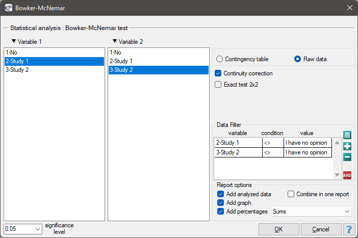
The settings window with the Bowker-McNemar test can be opened in Statistics menu → NonParametric tests → Bowker-McNemar or in ''Wizard''.

The Bowker test of internal symmetry

The Bowker test of internal symmetry (Bowker (1948)⁵⁾) is an extension of the McNemar test for 2 variables with more than 2 categories ( $c>2$ ). It is used to verify the hypothesis determining the symmetry of 2 results of measurements executed twice $X^{(1)}$ and $X^{(2)}$ of $X$ feature (symmetry of 2 dependent variables $X^{(1)}$ i $X^{(2)}$ ). An analysed feature may have more than 2 categories. The Bowker test of internal symmetry can be calculated on the basis of either raw data or a $c\times c$ contingency table.

$\begin{tabular}{|c|c||c|c|c|c|c|} \hline \multicolumn{2}{|c||}{Observed frequencies}& \multicolumn{5}{|c|}{$X^{(2)}$}\\\cline{3-7} \multicolumn{2}{|c||}{$O_{ij}$} & $X_1^{(2)}$ & $X_2^{(2)}$ & ... & $X_c^{(2)}$ & Total \\\hline \hline \multirow{5}{*}{$X^{(1)}$}& $X_1^{(1)}$ & $O_{11}$ & $O_{12}$ & ... & $O_{1c}$& $\sum_{j=1}^cO_{1j}$ \\\cline{2-7} & $X_2^{(1)}$ & $O_{21}$ & $O_{22}$ & ... & $O_{2c}$& $\sum_{j=1}^cO_{2j}$ \\\cline{2-7} & ...& ... & ... & ... & ...& ... \\\cline{2-7} & $X_c^{(1)}$ & $O_{c1}$ & $O_{c2}$ & ... & $O_{cc}$& $\sum_{j=1}^cO_{cj}$ \\\cline{2-7} & Total & $\sum_{i=1}^cO_{i1}$ & $\sum_{i=1}^cO_{i2}$ & ... & $\sum_{i=1}^cO_{ic}$& $n=\sum_{i=1}^c\sum_{j=1}^cO_{ij}$\\\hline \end{tabular}$

Hypotheses:

$\begin{array}{cl} \mathcal{H}_0: & O_{ij}=O_{ji},\\ \mathcal{H}_1: & O_{ij}\neq O_{ji} $ for at least one pair $ O_{ij}, O_{ji}, \end{array}$

where $j\neq i$ , $j\in{1,2,...,c}$ , $i\in{1,2,...,c}$ , so $O_{ij}$ and $O_{ji}$ are the frequencies of the symmetrical pairs in the $c\times c$ table

The test statistic is defined by:

$\begin{displaymath} \chi^2=\sum_{i=1}^c\sum_{j>i}\frac{(O_{ij}-O_{ji})^2}{O_{ij}+O_{ji}}. \end{displaymath}$

This statistic asymptotically (for large sample size) has the Chi-square distribution with a number of degrees of freedom calculated using the formula: $df=\frac{c(c-1)}{2}$ .

The p-value, designated on the basis of the test statistic, is compared with the significance level $\alpha$ :

$\begin{array}{ccl} $ if $ p \le \alpha & \Longrightarrow & $ reject $ \mathcal{H}_0 $ and accept $ \mathcal{H}_1, \\ $ if $ p > \alpha & \Longrightarrow & $ there is no reason to reject $ \mathcal{H}_0. \\ \end{array}$

EXAMPLE (opinion.pqs file)

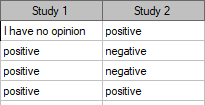
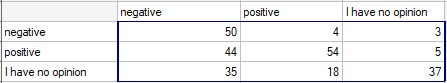
Two different surveys were carried out. They were supposed to analyse students' opinions about the particular academic professor. Both the surveys enabled students to give a positive opinion, a negative and a neutral one. Both surveys were carried out on the basis of the same sample of 250 students. But the first one was carried out the day before an exam done by the professor, and the other survey the day after the exam. There are some data below – in a form of raw rows, and all the data – in the form of a contingency table. Check, if both surveys give the similar results.

Hypotheses:

$\begin{array}{cl} \mathcal{H}_0: & $the number of students, who changed their opinions is exactly the same$\\ &$for each of the possibile symmetric opinion changes,$\\ \mathcal{H}_1: & $the number of students, who changed their opinions is different$\\ &$for at least one of the possibile symmetric opinion changes,$ \end{array}$

where, for example, changing the opinion from positive to negative one is symmetrical to changing the opinion from negative to positive one.

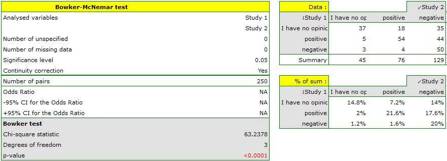
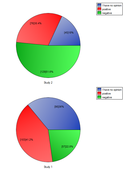
Comparing the p-value for the Bowker test (p-value<0.0001) with the significance level $\alpha=0.05$ it may be assumed that students changed their opinions. Looking at the table you can see that, there were more students who changed their opinions to negative ones after the exam, than those who changed it to positive ones after the exam. There were also students who did not evaluate the professor in the positive way after the exam any more.

If you limit your analysis only to the people having clear opinions about the professor (positive or negative ones), you can use the McNemar test:

Hypotheses:

$\begin{array}{cl} \mathcal{H}_0: & $the number of students, who changed their opinions from negative to positive ones$\\ &$ is exactly the same as those, who changed their opinions from positive to negative,$\\ \mathcal{H}_1: & $the number of students, who changed their opinions from negative to positive ones$\\ &$ is different from those, who changed their opinions from positive to negative.$ \end{array}$

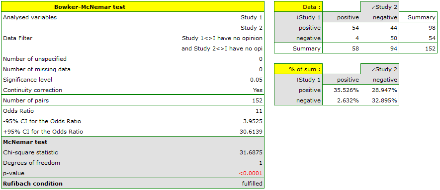
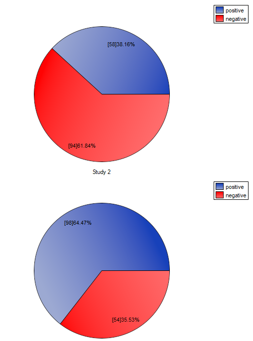
If you compare the p-value, calculated for the McNemar test (p-value < 0.0001), with the significance level $\alpha=0.05$ , you draw the conclusion that the students changed their opinions. There were much more students, who changed their opinions to negative ones after the exam, than those who changed their opinions to positive ones. The possibility of changing the opinion from positive (before the exam) to negative (after the exam) is eleven $\left(\frac{44}{4}\right)$ times greater than from negative to positive (the chance to change opinion in the opposite direction is: $\left(\frac{4}{44}\right)$ ).

¹⁾

McNemar Q. (1947), Note on the sampling error of the difference between correlated proportions or percentages. Psychometrika, 12, 153-157

²⁾

Rufibach K. (2010), Assessment of paired binary data; Skeletal Radiology volume 40, pages1–4

³⁾

Fagerland M.W., Lydersen S., and Laake P. (2013), The McNemar test for binary matched-pairs data: mid-p and asymptotic are better than exact conditional, BMC Med Res Methodol; 13: 91

⁴⁾

Liddell F.D.K. (1983), Simplified exact analysis of case-referent studies; matched pairs; dichotomous exposure. Journal of Epidemiology and Community Health; 37:82-84

⁵⁾

Bowker A.H. (1948), Test for symmetry in contingency tables. Journal of the American Statistical Association, 43, 572-574

PQStat - Baza Wiedzy

Narzędzia użytkownika

Narzędzia witryny

Pasek boczny

The McNemar test, the Bowker test of internal symmetry

Narzędzia strony