Narzędzia użytkownika
Narzędzia witryny
Pasek boczny
en:statpqpl:porown3grpl:nparpl:anova_kwpl
The Kruskal-Wallis ANOVA
The Kruskal-Wallis one-way analysis of variance by ranks (Kruskal 1952 1); Kruskal and Wallis 1952 2)) is an extension of the U-Mann-Whitney test on more than two populations. This test is used to verify the hypothesis that there is no shift in the compared distributions, i.e., most often the insignificant differences between medians of the analysed variable in ( ) populations (but you need to assume, that the variable distributions are similar - comparison of rank variances can be checked using Conover's rank test).
Additional analyses:
- it is possible to test for a trend in the arrangement of the groups under study by performing the Jonckheere-Terpstra test for trend.
Basic assumptions:
- measurement on an ordinal scale or on an interval scale,
Hypotheses:

where:
 distributions of the analysed variable of each population.
The test statistic is defined by:

where:
 ,
,
 – samples sizes
  ,
,
 – ranks ascribed to the values of a variable for
  , ,
, ,
 – correction for ties,
 – number of cases included in a tie.
The formula for the test statistic  includes the correction for ties
  . This correction is used, when ties occur (if there are no ties, the correction is not calculated, because of
  ).
).
The statistic asymptotically (for large sample sizes) has the Chi-square distribution with the number of degrees of freedom calculated using the formula:  .
.
The p-value, designated on the basis of the test statistic, is compared with the significance level  :
:

The POST-HOC tests
Introduction to the contrasts and the POST-HOC tests was performed in the unit, which relates to the one-way analysis of variance.
For simple comparisons, equal-size groups as well as unequal-size groups.
The Dunn test (Dunn 19643)) includes a correction for tied ranks (Zar 20104)) and is a test corrected for multiple testing. The Bonferroni or Sidak correction is most commonly used here, although other, newer corrections are also available, described in more detail in Multiple comparisons.
Example - simple comparisons (comparing 2 selected median / mean ranks with each other):

- [i] The value of critical difference is calculated by using the following formula:

where:
 - is the critical value (statistic) of the normal distribution for a given significance level corrected on the number of possible simple comparisons
  .
.
- [ii] The test statistic is defined by:

where:
 – mean of the ranks of the
  -th group, for ,
The formula for the test statistic  includes a correction for tied ranks. This correction is applied when tied ranks are present (when there are no tied ranks this correction is not calculated because
  ).
).
The test statistic asymptotically (for large sample sizes) has the normal distribution, and the p-value is corrected on the number of possible simple comparisons .
The non-parametric equivalent of Fisher LSD5), used for simple comparisons of both groups of equal and different sizes.
- [i] The value of critical difference is calculated by using the following formula:

where:

 is the critical value (statistic) Snedecor's F distribution for a given significance level and for degrees of freedom respectively: 1 i
  .
.
- [ii] The test statistic is defined by:

where:
– The mean ranks of the -th group, for ,
This statistic follows a t-Student distribution with degrees of freedom.
The settings window with the Kruskal-Wallis ANOVA can be opened in Statistics menu→NonParametric tests →Kruskal-Wallis ANOVA or in ''Wizard''.
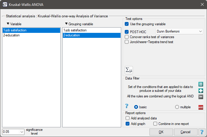
A group of 120 people was interviewed, for whom the occupation is their first job obtained after receiving appropriate education. The respondents rated their job satisfaction on a five-point scale, where:
1- unsatisfying job,
2- job giving little satisfaction,
3- job giving an average level of satisfaction,
4- job that gives a fairly high level of satisfaction,
5- job that is very satisfying.
We will test whether the level of reported job satisfaction does not change for each category of education.
Hypotheses:

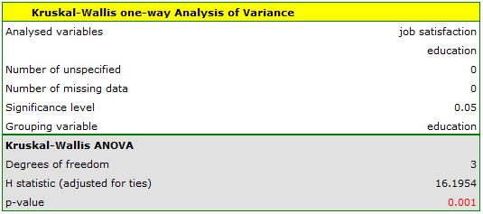
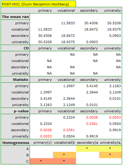
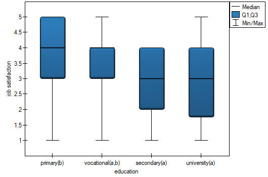
The obtained value of p=0.001 indicates a significant difference in the level of satisfaction between the compared categories of education. Dunn's POST-HOC analysis with Bonferroni's correction shows that significant differences are between those with primary and secondary education and those with primary and tertiary education. Slightly more differences can be confirmed by selecting the stronger POST-HOC Conover-Iman.
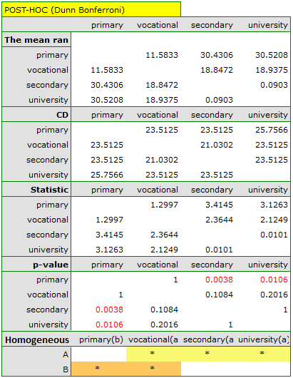
In the graph showing medians and quartiles we can see homogeneous groups determined by the POST-HOC test. If we choose to present Dunn's results with Bonferroni correction we can see two homogeneous groups that are not completely distinct, i.e. group (a) - people who rate job satisfaction lower and group (b)- people who rate job satisfaction higher. Vocational education belongs to both of these groups, which means that people with this education evaluate job satisfaction quite differently. The same description of homogeneous groups can be found in the results of the POST-HOC tests.
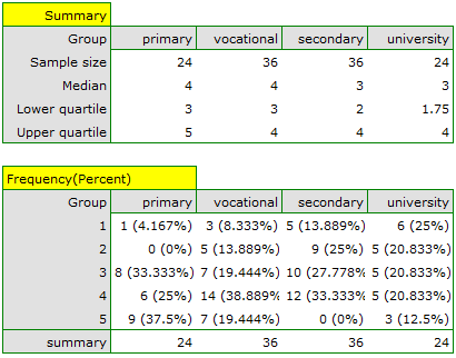
We can provide a detailed description of the data by selecting descriptive statistics in the analysis window  and indicating to add counts and percentages to the description.
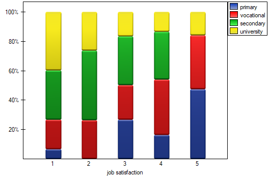
We can also show the distribution of responses in a column plot.
1)
Kruskal W.H., Wallis W.A. (1952), Use of ranks in one-criterion variance analysis. Journal of the American Statistical Association, 47, 583-621
4)
Zar J. H., (2010), Biostatistical Analysis (Fifth Editon). Pearson Educational
5)
Conover W. J. (1999), Practical nonparametric statistics (3rd ed). John Wiley and Sons, New York
en/statpqpl/porown3grpl/nparpl/anova_kwpl.txt · ostatnio zmienione: 2022/12/03 17:07 przez admin
Narzędzia strony
Wszystkie treści w tym wiki, którym nie przyporządkowano licencji, podlegają licencji: CC Attribution-Noncommercial-Share Alike 4.0 International
