Narzędzia użytkownika
Narzędzia witryny
Pasek boczny
en:statpqpl:korelpl
Spis treści
Correlation
{\ovalnode{A}{\hyperlink{rozklad_normalny}{\begin{tabular}{c}Are\\the data\\normally\\distributed?\end{tabular}}}}
\rput[br](2.9,6.2){\rnode{B}{\psframebox{\hyperlink{wspolczynnik_pearsona}{\begin{tabular}{c}tests for\\linear\\correlation\\coefficient $r_p$\\ and linear \\regression\\coefficient $\beta$\end{tabular}}}}}
\ncline[angleA=-90, angleB=90, arm=.5, linearc=.2]{->}{A}{B}
\rput(2.2,10.4){Y}
\rput(4.3,12.5){N}
\rput(7.5,14){\hyperlink{porzadkowa}{Ordinal scale}}
\rput[br](9.2,11.09){\rnode{C}{\psframebox{\hyperlink{wspolczynniki_monotoniczne}{\begin{tabular}{c}tests for\\monotonic\\correlation\\coefficients\\$r_s$ or $\tau$ \end{tabular}}}}}
\ncline[angleA=-90, angleB=90, arm=.5, linearc=.2]{->}{A}{C}
\rput(12.5,14){\hyperlink{nominalna}{Nominal scale}}
\rput[br](16.1,11.9){\rnode{D}{\psframebox{\hyperlink{wsp_tabel_kontyngencji}{\begin{tabular}{c}$\chi^2$ test and dedicated to them\\$C$, $\phi$, $V$ contingency coefficients\\or test for $Q$ contingency coefficient\end{tabular}}}}}
\rput(4,9.8){\hyperlink{testy_normalnosci}{normality tests}}
\psline[linestyle=dotted]{<-}(3.4,11.2)(4,10)
\end{pspicture}](/lib/exe/fetch.php?media=wiki:latex:/img5c5040e5eb96c39a53b4d9b209480adf.png "LaTeX")
The Correlation coefficients are one of the measures of descriptive statistics which represent the level of correlation (dependence) between 2 or more features (variables). The choice of a particular coefficient depends mainly on the scale, on which the measurements were done. Calculation of coefficients is one of the first steps of the correlation analysis. Then the statistic significance of the gained coefficients may be checked using adequate tests.
Note
Note, that the dependence between variables does not always show the cause-and-effect relationship.
Parametric tests
The linear correlation coefficients
The Pearson product-moment correlation coefficient  called also the Pearson's linear correlation coefficient (Pearson (1896,1900)) is used to decribe the strength of linear relations between 2 features. It may be calculated on an interval scale as long as there are no measurement outliers and the distribution of residuals or the distribution of the analyed features is a normal one.

where:
 - the following values of the feature
  and
and  ,
,
 - means values of features: and ,
 - sample size.
Note
 – the Pearson product-moment correlation coefficient in a population;
– the Pearson product-moment correlation coefficient in a sample.
The value of  , and it should be interpreted the following way:
 means a strong positive linear correlation – measurement points are closed to a straight line and when the independent variable increases, the dependent variable increases too;
 means a strong negative linear correlation – measurement points are closed to a straight line, but when the independent variable increases, the dependent variable decreases;
- if the correlation coefficient is equal to the value or very closed to zero, there is no linear dependence between the analysed features (but there might exist another relation - a not linear one).
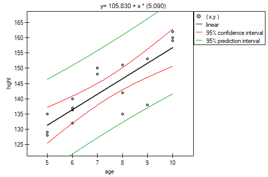
Graphic interpretation of .

If one out of the 2 analysed features is constant (it does not matter if the other feature is changed), the features are not dependent from each other. In that situation can not be calculated.
Note
You are not allowed to calculate the correlation coefficient if: there are outliers in a sample (they may make that the value and the sign of the coefficient would be completely wrong), if the sample is clearly heterogeneous, or if the analysed relation takes obviously the other shape than linear.
The coefficient of determination:  – reflects the percentage of a dependent variable a variability which is explained by variability of an independent variable.
A created model shows a linear relationship:

 and
and  coefficients of linear regression equation can be calculated using formulas:

EXAMPLE cont. (age-height.pqs file)
The Pearson correlation coefficient significance
The test of significance for Pearson product-moment correlation coefficient is used to verify the hypothesis determining the lack of linear correlation between an analysed features of a population and it is based on the Pearson's linear correlation coefficient calculated for the sample. The closer to 0 the value of coefficient is, the weaker dependence joins the analysed features.
Basic assumptions:
- measurement on the interval scale,
- normality of distribution of residuals or an analysed features in a population.
Hypotheses:

The test statistic is defined by:

where  .
.
The value of the test statistic can not be calculated when  or
or  or when
  .
.
The test statistic has the t-Student distribution with  degrees of freedom.
The p-value, designated on the basis of the test statistic, is compared with the significance level :

EXAMPLE cont. (age-height.pqs file)
The slope coefficient significance
The test of significance for the coefficient of linear regression equation
This test is used to verify the hypothesis determining the lack of a linear dependence between an analysed features and is based on the slope coefficient (also called an effect), calculated for the sample. The closer to 0 the value of coefficient is, the weaker dependence presents the fitted line.
Basic assumptions:
- measurement on the interval scale,
- normality of distribution of residuals or an analysed features in a population.
Hypotheses:

The test statistic is defined by:

where:
 ,
,
 ,
,
 – standard deviation of the value of features: and .
The value of the test statistic can not be calculated when or or when .
The test statistic has the t-Student distribution with degrees of freedom.
The p-value, designated on the basis of the test statistic, is compared with the significance level :
Prediction
is used to predict the value of a one variable (mainly a dependent variable  ) on the basis of a value of an another variable (mainly an independent variable
  ). The accuracies of a calculated value are defined by prediction intervals calculated for it.
- Interpolation is used to predict the value of a variable, which occurs inside the area for which the regression model was done. Interpolation is mainly a safe procedure - it is assumed only the continuity of the function of analysed variables.
- Extrapolation is used to predict the value of variable, which occurs outside the area for which the regression model was done. As opposed to interpolation, extrapolation is often risky and is performed only not far away from the area, where the regression model was created. Similarly to the interpolation, it is assumed the continuity of the function of analysed variables.
Analysis of model residuals - explanation in the Multiple Linear Regression module.
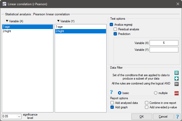
The settings window with the Pearson's linear correlation can be opened in Statistics menu→Parametric tests→linear correlation (r-Pearson) or in ''Wizard''.
Among some students of a ballet school, the dependence between age and height was analysed. The sample consists of 16 children and the following results of these features (related to the children) were written down:
(age, height): (5, 128) (5, 129) (5, 135) (6, 132) (6, 137) (6, 140) (7, 148) (7, 150) (8, 135) (8, 142) (8, 151) (9, 138) (9, 153) (10, 159) (10, 160) (10, 162).}
Hypotheses:

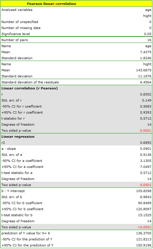
Comparing the  value < 0.0001 with the significance level
  , we draw the conclusion, that there is a linear dependence between age and height in the population of children attening to the analysed school. This dependence is directly proportional, it means that the children grow up as they are getting older.
The Pearson product-moment correlation coefficient, so the strength of the linear relation between age and height counts to =0.83. Coefficient of determination  means that about 69\% variability of height is explained by the changing of age.
From the regression equation:
 it is possible to calculate the predicted value for a child, for example: in the age of 6. The predicted height of such child is 136.37cm.
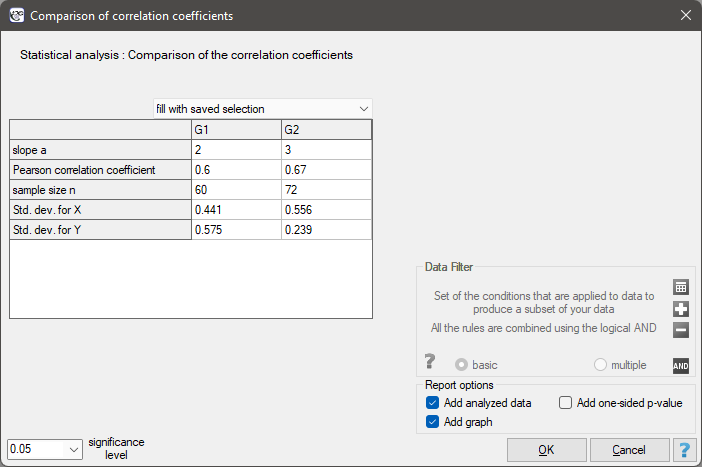
Comparison of correlation coefficients
The test for checking the equality of the Pearson product-moment correlation coefficients, which come from 2 independent populations
This test is used to verify the hypothesis determining the equality of 2 Pearson's linear correlation coefficients ( ,
,  .
.
Basic assumptions:
 and
and  describe the strength of dependence of the same features: and ,
- sizes of both samples (
 and
and  ) are known.
Hypotheses:

The test statistic is defined by:

where:
 ,
,
 .
.
The test statistic has the t-Student distribution with  degrees of freedom.
The p-value, designated on the basis of the test statistic, is compared with the significance level :
Note
A comparison of the slope coefficients of the regression lines can be made in a similar way. </WRAP>
Comparison of the slope of regression lines
The test for checking the equality of the coefficients of linear regression equation, which come from 2 independent populations
This test is used to verify the hypothesis determining the equality of 2 coefficients of the linear regression equation  and
and  in analysed populations.
Basic assumptions:
- and describe the strength of dependence of the same features: and ,
- both sample sizes ( and ) are known,
 and
and  ) are known,
Hypotheses:

The test statistic is defined by:

where:
 ,
,
 .
.
The test statistic has the t-Student distribution with degrees of freedom.
The p-value, designated on the basis of the test statistic, is compared with the significance level :
The settings window with the comparison of correlation coefficients can be opened in Statistics menu → Parametric tests → Comparison of correlation coefficients.
Non-parametric tests
The monotonic correlation coefficients
The monotonic correlation may be described as monotonically increasing or monotonically decreasing. The relation between 2 features is presented by the monotonic increasing if the increasing of the one feature accompanies with the increasing of the other one. The relation between 2 features is presented by the monotonic decreasing if the increasing of the one feature accompanies with the decreasing of the other one.
The Spearman's rank-order correlation coefficient  is used to describe the strength of monotonic relations between 2 features: and . It may be calculated on an ordinal scale or an interval one. The value of the Spearman's rank correlation coefficient should be calculated using the following formula:

 – difference of
  .
.
This formula is modified when there are ties:

where:
 ,
,  ,
, ,
,  ,
, – number of cases included in tie.
This correction is used, when ties occur. If there are no ties, the correction is not calculated, because the correction is reduced to the formula describing the above equation.
Note
 – the Spearman's rank correlation coefficient in a population;
– the Spearman's rank correlation coefficient in a sample.
The value of  , and it should be interpreted the following way:
 means a strong positive monotonic correlation (increasing) – when the independent variable increases, the dependent variable increases too;
 means a strong negative monotonic correlation (decreasing) – when the independent variable increases, the dependent variable decreases;
- if the Spearman's correlation coefficient is of the value equal or very close to zero, there is no monotonic dependence between the analysed features (but there might exist another relation - a non monotonic one, for example a sinusoidal relation).
The Kendall's tau correlation coefficient (Kendall (1938)1)) is used to describe the strength of monotonic relations between features . It may be calculated on an ordinal scale or interval one. The value of the Kendall's  correlation coefficient should be calculated using the following formula:

where:
 – number of pairs of observations, for which the values of the ranks for the feature as well as feature are changed in the same direction (the number of agreed pairs),
 – number of pairs of observations, for which the values of the ranks for the feature are changed in the different direction than for the feature (the number of disagreed pairs),
 ,
,  ,
,- – number of cases included in a tie.
The formula for the correlation coefficient includes the correction for ties. This correction is used, when ties occur (if there are no ties, the correction is not calculated, because of  i
i  ) .
) .
Note
 – the Kendall's correlation coefficient in a population;
– the Kendall's correlation coefficient in a sample.
The value of  , and it should be interpreted the following way:
 means a strong agreement of the sequence of ranks (the increasing monotonic correlation) – when the independent variable increases, the dependent variable increases too;
 means a strong disagreement of the sequence of ranks (the decreasing monotonic correlation) – when the independent variable increases, the dependent variable decreases;
- if the Kendall's correlation coefficient is of the value equal or very close to zero, there is no monotonic dependence between analysed features (but there might exist another relation - a non monotonic one, for example a sinusoidal relation).
Spearman's versus Kendall's coefficient
- for an interval scale with a normality of the distribution, the gives the results which are close to , but may be totally different from ,
- the value is less or equal to value,
- the is an unbiased estimator of the population parameter , while the is a biased estimator of the population parameter .
EXAMPLE cont. (sex-height.pqs file)
The Spearman's rank-order correlation coefficient
The test of significance for the Spearman's rank-order correlation coefficient is used to verify the hypothesis determining the lack of monotonic correlation between analysed features of the population and it is based on the Spearman's rank-order correlation coefficient calculated for the sample. The closer to 0 the value of coefficient is, the weaker dependence joins the analysed features.
Basic assumptions:
- measurement on an ordinal scale or on an interval scale.
Hypotheses:

The test statistic is defined by:

where  .
.
The value of the test statistic can not be calculated when  lub
lub  or when .
The test statistic has the t-Student distribution with degrees of freedom.
The p-value, designated on the basis of the test statistic, is compared with the significance level :
The settings window with the Spearman's monotonic correlation can be opened in Statistics menu → NonParametric tests→monotonic correlation (r-Spearman) or in ''Wizard''.

The effectiveness of a new therapy designed to lower cholesterol levels in the LDL fraction was studied. 88 people at different stages of the treatment were examined. We will test whether LDL cholesterol levels decrease and stabilize with the duration of the treatment (time in weeks).
Hypotheses:


Comparing <0.0001 with a significance level we find that there is a statistically significant monotonic relationship between treatment time and LDL levels. This relationship is initially decreasing and begins to stabilize after 150 weeks. The Spearman's monotonic correlation coefficient and therefore the strength of the monotonic relationship for this relationship is quite high at =-0.78. The graph was plotted by curve fitting through local LOWESS linear smoothing techniques.

The Kendall's tau correlation coefficient
The test of significance for the Kendall's correlation coefficient is used to verify the hypothesis determining the lack of monotonic correlation between analysed features of population. It is based on the Kendall's tau correlation coefficient calculated for the sample. The closer to 0 the value of tau is, the weaker dependence joins the analysed features.
Basic assumptions:
- measurement on an ordinal scale or on an interval scale.
Hypotheses:

The test statistic is defined by:

The test statistic asymptotically (for a large sample size) has the normal distribution.
The p-value, designated on the basis of the test statistic, is compared with the significance level :
The settings window with the Kendall's monotonic correlation can be opened in Statistics menu → NonParametric tests→monotonic correlation (tau-Kendall) or in ''Wizard''.
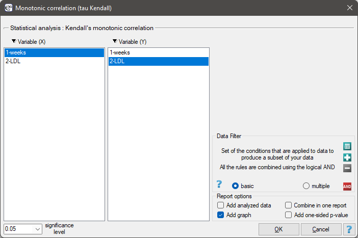
EXAMPLE cont. (LDL weeks.pqs file)
Hypotheses:
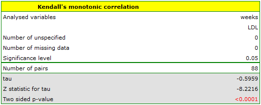
Comparing p<0.0001 with a significance level we find that there is a statistically significant monotonic relationship between treatment time and LDL levels. This relationship is initially decreasing and begins to stabilize after 150 weeks. The Kendall's monotonic correlation coefficient, and therefore the strength of the monotonic relationship for this relationship is quite high at =-0.60. The graph was plotted by curve fitting through local LOWESS linear smoothing techniques.
Contingency tables coefficients and their statistical significance
The contingency coefficients are calculated for the raw data or the data gathered in a contingency table.
The settings window with the measures of correlation can be opened in Statistics menu → NonParametric tests → Ch-square, Fisher, OR/RR option Measures of dependence… or in ''Wizard''.
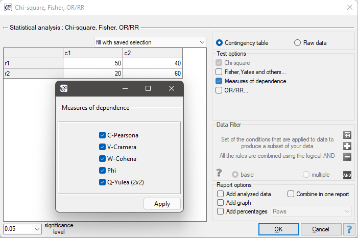
The Yule's Q contingency coefficient
The Yule's  contingency coefficient (Yule, 19002)) is a measure of correlation, which can be calculated for
  contingency tables.

where:
 - observed frequencies in a contingency table.
The coefficient value is included in a range of  . The closer to 0 the value of the is, the weaker dependence joins the analysed features, and the closer to
  1 or +1, the stronger dependence joins the analysed features. There is one disadvantage of this coefficient. It is not much resistant to small observed frequencies (if one of them is 0, the coefficient might wrongly indicate the total dependence of features).
The statistic significance of the Yule's coefficient is defined by the  test.
test.
Hypotheses:

The test statistic is defined by:

The test statistic asymptotically (for a large sample size) has the normal distribution.
The p-value, designated on the basis of the test statistic, is compared with the significance level :
The Phi contingency coefficient is a measure of correlation, which can be calculated for contingency tables.

The  coefficient value is included in a range of
  . The closer to 0 the value of is, the weaker dependence joins the analysed features, and the closer to 1, the stronger dependence joins the analysed features.
The contingency coefficient is considered as statistically significant, if the p-value calculated on the basis of the  test (designated for this table) is equal to or less than the significance level .
The Cramer's V contingency coefficient
The Cramer's V contingency coefficient (Cramer, 19463)), is an extension of the coefficient on  contingency tables.

where:
Chi-square – value of the test statistic,
– total frequency in a contingency table,
 – the smaller the value out of
  and
and  .
.
The  coefficient value is included in a range of . The closer to 0 the value of is, the weaker dependence joins the analysed features, and the closer to 1, the stronger dependence joins the analysed features. The coefficient value depends also on the table size, so you should not use this coefficient to compare different sizes of contingency tables.
The contingency coefficient is considered as statistically significant, if the p-value calculated on the basis of the test (designated for this table) is equal to or less than the significance level .
W-Cohen contingency coefficient
The  -Cohen contingency coefficient (Cohen (1988)4)), is a modification of the V-Cramer coefficient and is computable for tables.

where:
Chi-square – value of the test statistic,
– total frequency in a contingency table,
– the smaller the value out of and .
The coefficient value is included in a range of  , where
  (for tables where at least one variable contains only two categories, the value of the coefficient is in the range ). The closer to 0 the value of is, the weaker dependence joins the analysed features, and the closer to
  , the stronger dependence joins the analysed features. The coefficient value depends also on the table size, so you should not use this coefficient to compare different sizes of contingency tables.
The contingency coefficient is considered as statistically significant, if the p-value calculated on the basis of the test (designated for this table) is equal to or less than the significance level .
The Pearson's C contingency coefficient
The Pearson's  contingency coefficient is a measure of correlation, which can be calculated for contingency tables.

The coefficient value is included in a range of  . The closer to 0 the value of is, the weaker dependence joins the analysed features, and the farther from 0, the stronger dependence joins the analysed features. The coefficient value depends also on the table size (the bigger table, the closer to 1 value can be), that is why it should be calculated the top limit, which the coefficient may gain – for the particular table size:

where:
– the smaller value out of and .
An uncomfortable consequence of dependence of value on a table size is the lack of possibility of comparison the coefficient value calculated for the various sizes of contingency tables. A little bit better measure is a contingency coefficient adjusted for the table size ( ):
):

The contingency coefficient is considered as statistically significant, if the p-value calculated on the basis of the test (designated for this table) is equal to or less than significance level .
EXAMPLE (sex-exam.pqs file)
There is a sample of 170 persons ( ), who have 2 features analysed (=sex, =passing the exam). Each of these features occurs in 2 categories (
 =f,
=f,  =m,
=m,  =yes,
=yes,  =no). Basing on the sample, we would like to get to know, if there is any dependence between sex and passing the exam in an analysed population. The data distribution is presented in a contingency table:}

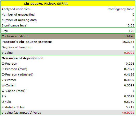
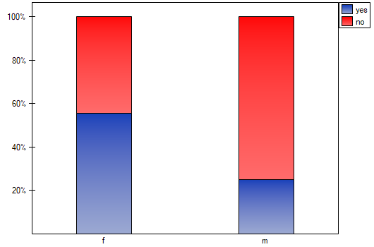
The test statistic value is  and the value calculated for it: p<0.0001. The result indicates that there is a statistically significant dependence between sex and passing the exam in the analysed population.
Coefficient values, which are based on the test, so the strength of the correlation between analysed features are:
-Pearson = 0.42.
-Cramer = = -Cohen = 0.31
The -Yule = 0.58, and the value of the test (similarly to test) indicates the statistically significant dependence between the analysed features.
1)
Kendall M.G. (1938), A new measure of rank correlation. Biometrika, 30, 81-93
2)
Yule G. (1900), On the association of the attributes in statistics: With illustrations from the material ofthe childhood society, and c. Philosophical Transactions of the Royal Society, Series A, 194,257-3 19
3)
Cramkr H. (1946), Mathematical models of statistics. Princeton, NJ: Princeton University Press
4)
Cohen J. (1988), Statistical Power Analysis for the Behavioral Sciences, Lawrence Erlbaum Associates, Hillsdale, New Jersey
en/statpqpl/korelpl.txt · ostatnio zmienione: 2022/02/13 18:28 przez admin
Narzędzia strony
Wszystkie treści w tym wiki, którym nie przyporządkowano licencji, podlegają licencji: CC Attribution-Noncommercial-Share Alike 4.0 International
