Spis treści

Survival analysis

Survival analysis

Survival analysis is often used in medicine. In other fields of study it is also called reliability analysis, duration analysis, or event history analysis. Its main goal is to evaluate the remaining time of the survival of, for example, patients after an operation. Its main purpose is to evaluate the survival time of e.g. patients after surgery - the tools used here are life tables and Kaplan-Meier curves. Another interesting aspect is the comparison of survival times e.g. survival times after different treatments - for this purpose methods of comparing 2 or more survival curves are used. A number of methods (regression models) have also been developed to study the influence of various variables on survival time.

To help understand the issue, basic definitions will be given using an example describing the life expectancy of heart transplant patients:

Event – is the change interesting to the researcher, e.g. death;
Survival time – is the period of time between the initial state and the occurrence of a given event, e.g. the length of a patient's life after a heart transplantation.

Note

In the analysis one column with the calculated time ought to be marked. When we have at our disposal two points in time: the initial and the final ones, before the analysis we calculate the time between the two points, using the datasheet formulas.

Censored observations – are the observations for which we only have incomplete pieces of information about the survival time.

Censored and complete observations – an example concerning the survival time after a heart transplantation:

a complete observation – we know the date of the transplantation and the date of the patient's death so we can establish the exact survival time after the transplantation.
observation censored on the right side – the date of the patient's death is not known (the patient is alive when the study finishes) so the exact survival time cannot be established.
observation censored on the left side – the date of the heart transplantation is not known but we know it was before this study started, and we cannot establish the exact survival time.

$\begin{pspicture}(-5,-.7)(7,5.6) \psline{->}(0,0)(0,5) \psline{->}(0,0)(8.3,0) \psline{-}(1,0)(1,4.8) \psline{-}(6,0)(6,4.8) \psline[linecolor=green, linewidth=2pt]{->}(2,4)(5,4) \psline[linecolor=red, linewidth=2pt]{->}(1,2.5)(7,2.5) \psline[linecolor=red, linewidth=2pt]{->}(0.3,1)(4,1) \rput(1,-.3){beginning} \rput(1,-.7){of the study} \rput(6,-.3){end} \rput(6,-.7){of the study} \rput(8.1,-.3){time} \end{pspicture}$

Note

The end of the study means the end of the observation of the patient. It is not always the same moment for all patients. It can be the moment of losing touch with the patient (so we do not now the patient's survival time). Analogously, the beginning of the study does not have to be the same point in time for all patients.

Life tables

The window with settings for life tables is accessed via the menu Advanced statistics→Survival analysis→Life tables

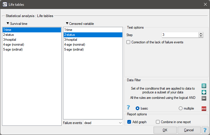
Life tables are created for time ranges with equal spans, provided by the researcher. The ranges can be defined by giving the step. For each range PQStat calculates:

the number of entered cases – the number of people who survived until the time defined by the range;
the number of censored cases – the number of people in a given range qualified as censored cases;
the number of cases at risk – the number of people in a given range minus a half of the censored cases in the given range;
the number of complete cases – the number of people who experienced the event (i.e. died) in a given range;
proportions of complete cases – the proportion of the number of complete cases (deaths) in a given range to the number of the cases at risk in that range;
proportions of the survival cases – calculated as 1 minus the proportion of complete cases in a given range;
cumulative survival proportion (survival function) – the probability of surviving over a given period of time. Because to survive another period of time, one must have survived all the previous ones, the probability is calculated as the product of all the previous proportions of the survival cases.

$\pm$ standard error of the survival function;

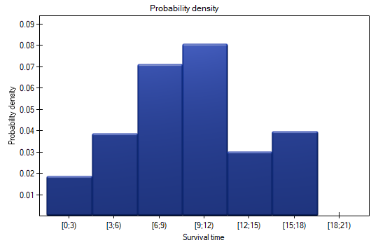
probability density – the calculated probability of experiencing the event (death) in a given range, calculated in a period of time;

$\pm$ standard error of the probability density;

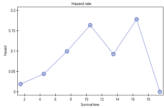
hazard rate – probability (calculated per a unit of time) that a patient who has survived until the beginning of a given range will experience the event (die) in that range;

$\pm$ standard error of the hazard rate

Note

In the case of a lack of complete observations in any range of survival time range there is the possibility of using correction. The zero number of complete cases is then replaced with value 0.5.

Graphic interpretation

We can illustrate the information obtained thanks to the life tables with the use of several charts:

a cumulative survival proportion graph,
a probability density graph,
a hazard rate graph.

Example (transplant.pqs file)

Patients' survival rate after the transplantation of a liver was studied. 89 patients were observed over 21 years. The age of a patient at the time of the transplantation was in the range of $\langle 45$ years $; 60$ years $)$ . A fragment of the collected data is presented in the table below:

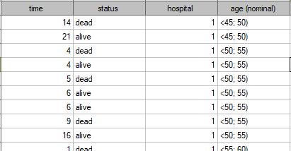
The complete data in the analysis are those as to which we have complete information about the length of life after the transplantation, i.e. described as „death” (it concerns 53 people which constitutes 59.55% of sample). The censored data are those about which we do not have that information because at the time when the study was finished the patients were alive (36 people, i.e. 40.45% of them). We build the life tables of those patients by creating time periods of 3 years:

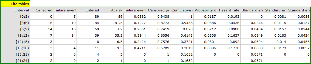
For each 3-year period of time we can interpret the results obtained in the table, for example, for people living for at least 9 years after the transplantation who are included in the range [9;12): \item the number of people who survived 9 years after the transplantation is 39, \item there are 7 people about whom we know they had lived at least 9-12 years at the moment the information about them was gathered but we do not know if they lived longer as they were left out of the study after that time, \item the number of people at the risk of death in that age range is 36, \item there are 14 people about whom we know they died 9 to 12 years after the transplantation, \item 39.4% of the endangered patients died 9 to 12 years after the transplantation, \item 60.6% of the endangered patients lived 9 to 12 years after the transplantation, \item the percent of survivors 9 years after the transplantation is 61.4% $\pm$ 5%, \item 0,08 $\pm$ 0.02 is the death probability for each year from the 9-12 range. The results will be presented on a few graphs:

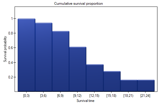
The probability of survival decreases with the time passed since the transplantation. We do not, however, observe a sudden plunge of the survival function, i.e. a period of time in which the probability of death would rise dramatically.

2022/02/09 12:56

Kaplan-Meier curves

Kaplan-Meier curves allow the evaluation of the survival time without the need to arbitrarily group the observations like in the case of life tables. The estimator was introduced by Kaplan and Meier (1958)\cite{kaplan}.

The window with settings for Kaplan-Meier curve is accessed via the menu Advanced statistics→Survival analysis→Kaplan-Meier Analysis

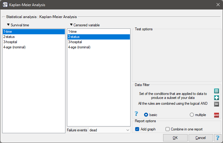
As with survival tables we calculate the survival function, i.e. the probability of survival until a certain time. The graph of the Kaplan-Meier survival function is created by a step function. Based on the standard error (Greenwood formula) and the logarithmic transformation (log-log), confidence intervals around this curve are constructed. The point of time at which the value of the function is 0.5 is the survival time median. The median indicates 50% risk of mortality, it means we can expect that half of the patients will die within a specific time. Both the median and other percentiles are determined as the shortest survival time for which the survival function is smaller or equal to a given percentile. For the median, a confidence interval is determined based on the test-based method by Brookmeyer and Crowley (1982)\cite{brookmeyer}. The survival time mean is determined as the field under the survival curve.

The data concerning the survival time are usually very heavily skewed so in the survival analysis the median is a better measure of the central tendency than the mean.

EXAMPLE (transplant.pqs file)

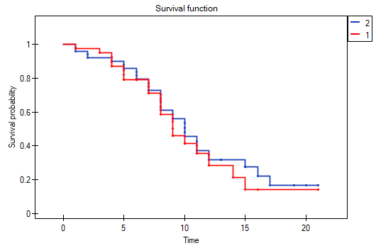
We present the survival time after a liver transplantation, with the use of the Kaplan-Meier curve

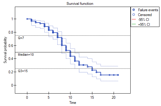
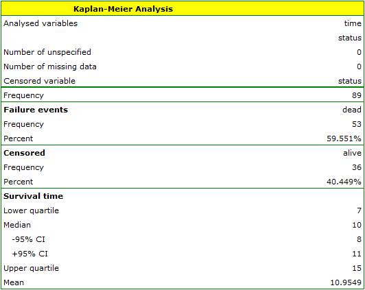
The survival function does not suddenly plunge right after the transplantation. Therefore, we conclude that the initial period after the transplantation does not carry a particular risk of death. The value of the median shows that within 10 years after the transplant, we expect that half of the patients will die. The value is marked on the graph by drawing a line in point 0.5 which signifies the median. In a similar manner we mark the quartiles in the graph.

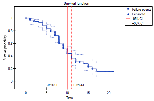
We can visualize the confidence interval for the median on a graph by drawing vertical lines based on the confidence interval around the curve and lines at the 0.5 level.

2022/02/09 12:56

Comparison of survival curves

The survival functions can be built separately for different subgroups, e.g. separately for women and men, and then compared. Such a comparison may concern two curves or more.

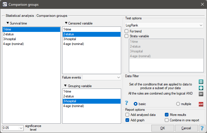
The window with settings for the comparison of survival curves is accessed via the menu Advanced statistics→Survival analysis→Comparison groups

Comparisons of $k$ survival curves $S_1,S_2,...,S_k$ , at particular points of the survival time $t$ , in the program can be made with the use of three tests:

Log-rank test the most popular test drawing on the Mantel-Heanszel procedure for many 2 x 2 tables (Mantel-Heanszel 1959¹⁾, Mantel 1966²⁾, Cox 1972³⁾),

Gehan's generalization of Wilcoxon's test deriving from Wilcoxon's test (Breslow 1970, Gehan 1965⁴⁾⁵⁾),

Tarone-Ware test deriving from Wilcoxon's test (Tarone and Ware 1977⁶⁾).

The three tests are based on the same test statistic, they only differ in weights $w_j$ the particular points of the timeline on which the test statistic is based.

Log-rank test: $w_j=1$ – all the points of the timeline have the same weight which gives the later values of the timeline a greater influence on the result;

Gehan's generalization of Wilcoxon's test: $w_j=n_j$ – time moments are weighted with the number of observations in each of them, so greater weights are ascribed to the initial values of the time line;

Tarone-Ware test: $w_j=\sqrt{n_j}$ – time moments are weighted with the root of the number of observations in each of them, so the test is situated between the two tests described earlier.

An important condition for using the tests above is the proportionality of hazard. Hazard, defined as the slope of the survival curve, is the measure of how quickly a failure event takes place. Breaking the principle of hazard proportionality does not completely disqualify the tests above but it carries some risks. First of all, the placement of the point of the intersection of the curves with respect to the timeline has a decisive influence on decreasing the power of particular tests.

EXAMPLE cont. (transplant.pqs file)

Differences among the survival curves

Hypotheses:

$\begin{array}{ll} \mathcal{H}_0: & S_1(t)=S_2(t)=...=S_k(t),$\quad for all $t,\\ \mathcal{H}_1: & $not all $S_i(t)$ are equal$. \end{array}$

In calculations was used chi-square statistics form:

$\begin{displaymath} \chi^2=U'V^{-1}U \end{displaymath}$

where:

$U_i=\sum_{j=1}^{m}w_j(d_{ij}-e_{ij})$

$V$ - covariance matrix of dimensions $(k-1)\times(k-1)$

where:

diagonal: $\sum_{j=1}^{m}w_j^2\frac{n_{ij}(n_j-n_{ij})d_j(n_j-d_j)}{n^2_j(n_j-1)}$ ,

off diagonal: $\sum_{j=1}^{m}w_j^2\frac{n_{ij}n_{lj}d_j(n_j-d_j)}{n^2_j(n_j-1)}$

$m$ – number of moments in time with failure event (death),

$d_j=\sum_{i=1}^k d_{ij}$ – observed number of failure events (deaths) in the $j$ -th moment of time,

$d_{ij}$ – observed number of failure events (deaths) in the w $i$ -th group w in the $j$ -th moment of time,

$e_{ij}=\frac{n_{ij}d_j}{n_j}$ – expected number of failure events (deaths) in the w $i$ -th group w in the $j$ -th moment of time,

$n_j=\sum_{i=1}^k n_{ij}$ – the number of cases at risk in the $j$ -th moment of time.

The statistic asymptotically (for large sizes) has the Chi-square distribution with $df=k-1$ degrees of freedom.

The p-value, designated on the basis of the test statistic, is compared with the significance level $\alpha$ :

$\begin{array}{ccl} $ if $ p \le \alpha & \Longrightarrow & $ reject $ \mathcal{H}_0 $ and accept $ \mathcal{H}_1, \\ $ if $ p > \alpha & \Longrightarrow & $ there is no reason to reject $ \mathcal{H}_0. \\ \end{array}$

Hazard ratio

In the log-rank test the observed values of failure events (deaths) $O_i=\sum_{j=1}^m d_{ij}$ and the appropriate expected values $E_i=\sum_{j=1}^m e_{ij}$ are given.

The measure for describing the size of the difference between a pair of survival curves is the hazard ratio ( $HR$ ).

$\begin{displaymath} HR= \frac{O_1/E_1}{O_2/E_2} \end{displaymath}$

If the hazard ratio is greater than 1, e.g. $HR=2$ , then the degree of the risk of a failure event in the first group is twice as big as in the second group. The reverse situation takes place when $HR$ is smaller than one. When $HR$ is equal to 1 both groups are equally at risk.

Note

The confidence interval for $HR$ is calculated on the basis of the standard deviation of the $HR$ logarithm (Armitage and Berry 1994⁷⁾).

EXAMPLE cont. (transplant.pqs file)

2022/02/09 12:56

Survival curves trend

Hypotheses:

$\begin{array}{ll} \mathcal{H}_0: & $In the studied population there is no trend in the placement of the $S_1,S_2,...,S_k$ curves,$\\ \mathcal{H}_1: & $In the studied population there is a trend in in the placement of the $S_1,S_2,...,S_k$ curves.$ \end{array}$

In the calculation the chi-square statistic was used, in the following form: $\begin{displaymath} \chi^2=\frac{(c'U)^2}{c'Vc} \end{displaymath}$

where:

$c=(c_1,c_2,...,c_k)$ – vector of the weights for the compared groups, informing about their natural order (usually the subsequent natural numbers).

The statistic asymptotically (for large sizes) has the Chi-square distribution with $1$ degree of freedom.

The p-value, designated on the basis of the test statistic, is compared with the significance level $\alpha$ :

$\begin{array}{ccl} $ if $ p \le \alpha & \Longrightarrow & $ reject $ \mathcal{H}_0 $ and accept $ \mathcal{H}_1, \\ $ if $ p > \alpha & \Longrightarrow & $ there is no reason to reject $ \mathcal{H}_0. \\ \end{array}$

In order to conduct a trend analysis in the survival curves the grouping variable must be a numerical variable in which the values of the numbers inform about the natural order of the groups. The numbers in the analysis are treated as the $c_1,c_2,...,c_k$ weights.

EXAMPLE cont. (transplant.pqs file)

2022/02/09 12:56

Survival curves for the stratas

Often, when we want to compare the survival times of two or more groups, we should remember about other factors which may have an impact on the result of the comparison. An adjustment (correction) of the analysis by such factors can be useful. For example, when studying rest homes and comparing the length of the stay of people below and above 80 years of age, there was a significant difference in the results. We know, however, that sex has a strong influence on the length of stay and the age of the inhabitants of rest homes. That is why, when attempting to evaluate the impact of age, it would be a good idea to stratify the analysis with respect to sex.

Hypotheses for the differences in survival curves:

$\begin{array}{ll} \mathcal{H}_0: & S_1^*(t)=S_2^*(t)=...=S_k^*(t),$\quad for all $t,\\ \mathcal{H}_1: & $not all $S_i^*(t)$ are equal$. \end{array}$

Hypotheses for the analysis of trends in survival curves:

$\begin{array}{ll} \mathcal{H}_0: & $In the studied population there is no trend in the placement of the $S_1^*,S_2^*,...,S_k^*,$ curves,$\\ \mathcal{H}_1: & $In the studied population there is a trend in in the placement of the $S_1^*,S_2^*,...,S_k^*$ curves$. \end{array}$

where $S_1^*(t), S_2^*(t), ..., S_k^*(t)$ -are the survival curves after the correction by the variable determining the strata.

The calculations for test statistics are based on formulas described for the tests, not taking into account the strata, with the difference that matrix U and V is replaced with the sum of matrices $\sum_{l=1}^L U$ and $\sum_{l=1}^L V$ . The summation is made according to the strata created by the variables with respect to which we adjust the analysis l={1,2,…,L}

The p-value, designated on the basis of the test statistic, is compared with the significance level $\alpha$ :

$\begin{array}{ccl} $ if $ p \le \alpha & \Longrightarrow & $ reject $ \mathcal{H}_0 $ and accept $ \mathcal{H}_1, \\ $ if $ p > \alpha & \Longrightarrow & $ there is no reason to reject $ \mathcal{H}_0. \\ \end{array}$

EXAMPLE cont. (transplant.pqs file)

The differences for two survival curves

Liver transplantations were made in two hospitals. We will check if the patients' survival time after transplantations depended on the hospital in which the transplantations were made. The comparisons of the survival curves for those hospitals will be made on the basis of all tests proposed in the program for such a comparison.

Hypotheses:

$\begin{array}{ll} \mathcal{H}_0: & $the survival curve of the patients of hospital no. 1 $=$ the survival curve of the patients of hospital no. 2$,\\ \mathcal{H}_1: & $the survival curve of the patients of hospital no. 1 $\neq $ the survival curve of the patients of hospital no. 2$. \end{array}$

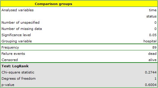
On the basis of the significance level $\alpha=0.05$ , based on the obtained value p=0.6004 for the log-rank test (p=0.6959 for Gehan's and 0.6465 for Tarone-Ware) we conclude that there is no basis for rejecting the hypothesis $\mathcal{H}_0$ . The length of life calculated for the patients of both hospitals is similar.

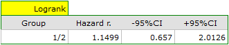
The same conclusion will be reached when comparing the risk of death for those hospitals by determining the risk ratio. The obtained estimated value is HR=1.1499 and 95% of the confidence interval for that value contains 1: $\langle$ 0.6570, 2.0126 $\rangle$ .

Differences for many survival curves

Liver transplantations were made for people at different ages. 3 age groups were distinguished: $\langle 45$ years $; 50$ years $<latex>$)$$ </latex>, $\langle 50$ years $; 55$ years $)$ , $\langle 55$ years $; 60$ years $)$ . We will check if the patients' survival time after transplantations depended on their age at the time of the transplantation.

Hypotheses:

$\begin{array}{ll} \mathcal{H}_0: & $survival rates of patients aged $\langle 45 $ years$; 50 $ years$), \langle 50 $ years$; 55 $ years$), \langle 55 $ years$; 60 $ years$)\\ & $are similar,$\\ \mathcal{H}_1: & $at least one survival curve out of the 3 curves above$\\ & $differs from the other curves.$\\ \end{array}$

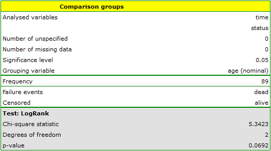
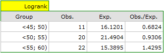
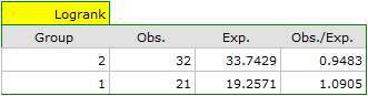
On the basis of the significance level $\alpha=0.05$ , based on the obtained value p=0.0692 in the log-rank test (p=0.0928 for Gehan's and p=0.0779 for Tarone-Ware) we conclude that there is no basis for the rejection of the hypothesis $\mathcal{H}_0$ . The length of life calculated for the patients in the three compared age groups is similar. However, it is noticeable that the values are quite near to the standard significance level 0.05.

When examining the hazard values (the ratio of the observed values and the expected failure events) we notice that they are a little higher with each age group (0.68, 0.93, 1.43). Although no statistically significant differences among them are seen it is possible that a growth trend of the hazard value (trend in the position of the survival rates) will be found.

Trend for many survival curves

If we introduce into the test the information about the ordering of the compared categories (we will use the age variable in which the age ranges will be numbered, respectively, 1, 2, and 3), we will be able to check if there is a trend in the compared curves. We will study the following hypotheses:

$\begin{array}{ll} \mathcal{H}_0: & $a lack of a trend in the survival time curves of the patients after a transplantation$\\ & $(a trend dependent on the age of the patients at the time of a transplantation),$\\ \mathcal{H}_1: & $the older the patients at the time of a transplantation, the greater/smaller$\\ & $ the probability of their survival over a given period of time.$\\ \end{array}$

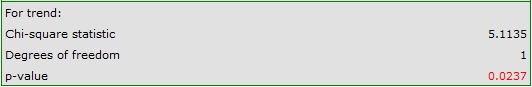
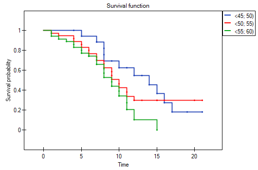
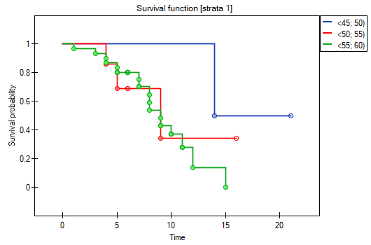
On the basis of the significance level $\alpha=0.05$ , based on the obtained value p=0.0237 in the log-rank test (p=0.0317 for Gehan's and p=0.0241 for Tarone-Ware) we conclude that the survival curves are positioned in a certain trend. On the Kaplan-Meier graph the curve for people aged $<latex>$\langle$$ </latex>55 years; 60 years) is the lowest. Above that curve there is the curve for patients aged $\langle$ 50 years; 55 years). The highest curve is the one for patients aged $\langle$ 45 years; 50 years). Thus, the older the patient at the time of a transplantation, the lower the probability of survival over a certain period of time.

Survival curves for stratas

Let us now check if the trend observed before is independent of the hospital in which the transplantation took place. For that purpose we will choose a hospital as the stratum variable.

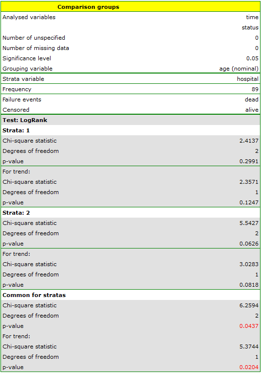
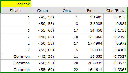
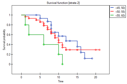
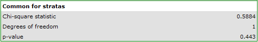
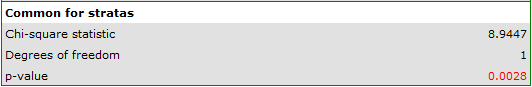
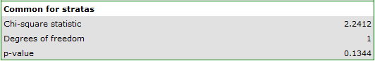
The report contains, firstly, an analysis of the strata: both the test results and the hazard ratio. In the first stratum the growing trend of hazard is visible but not significant. In the second stratum a trend with the same direction (a result bordering on statistical significance) is observed. A cumulation of those trends in a common analysis of strata allowed the obtainment of the significance of the trend of the survival curves. Thus, the older the patient at the time of a transplantation, the lower the probability of survival over a certain period of time, independently from the hospital in which the transplantation took place.

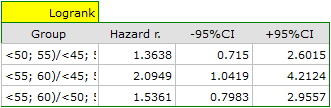
A comparative analysis of the survival curves, corrected by strata, yields a result significant for the log-rank and Tarone-Ware tests and not significant for Gehan's test, which might mean that the differences among the curves are not so visible in the initial survival periods as in the later ones. By looking at the hazard ratio of the curves compared in pairs

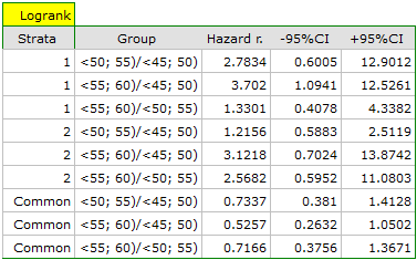
we can localize significant differences. For the comparison of the curve of the youngest group with the curve of the oldest group the hazard ratio is the smallest, 0.53, the 95\% confidence interval for that ratio, $\langle$ 0.26 ; 1.05 $\rangle$ , does contain value 1 but is on the verge of that value, which can suggest that there are significant differences between the respective curves. In order to confirm that supposition an inquisitive researcher can, with the use of the data filter in the analysis window, compare the curves in pairs.

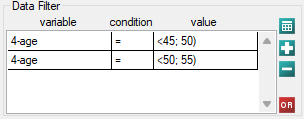
However, it ought to be remembered that one of the corrections for multiple comparisons should be used and the significance level should be modified. In this case, for Bonferroni's correction, with three comparisons, the significance level will be 0.017. For simplicity, we will only avail ourselves of the log-rank test.

$\langle$ 45 lat; 50 lat) vs $\langle$ 50 lat; 55 lat)

$\langle$ 45 lat; 50 lat) vs $\langle$ 55 lat; 60 lat)

$\langle$ 50 lat; 55 lat) vs $\langle$ 55 lat; 60 lat)

As expected, statistically significant differences only concern the survival curves of the youngest and oldest groups.

2022/02/09 12:56

Cox proportional hazard regression

The window with settings for Cox regression is accessed via the menu Advanced statistics→Survival analysis→Cox PH regression

Cox regression, also known as the Cox proportional hazard model (Cox D.R. (1972)⁸⁾), is the most popular regressive method for survival analysis. It allows the study of the impact of many independent variables ( $X_1$ , $X_2$ , $\ldots$ , $X_k$ ) on survival rates. The approach is, in a way, non-parametric, and thus encumbered with few assumptions, which is why it is so popular. The nature or shape of the hazard function does not have to be known and the only condition is the assumption which also pertains to most parametric survival models, i.e. hazard proportionality.

The function on which Cox proportional hazard model is based describes the resulting hazard and is the product of two values only one of which depends on time ( $t$ ):

$\begin{displaymath} h(t,X_1,X_2,...,X_k)=h_0(t)\cdot \exp\left(\sum_{i=1}^k\beta_iX_i\right), \end{displaymath}$

where:

$h(t,X_1,X_2,...,X_k)$ - the resulting hazard describing the risk changing in time and dependent on other factors, e.g. the treatment method,
$h_0(t)$ - the baseline hazard, i.e. the hazard with the assumption that all the explanatory variables are equal to zero,

$\sum_{i=1}^k\beta_iX_i$ - a combination (usually linear) of independent variables and model parameters,

$X_1,X_2,\ldots X_k$ - explanatory variables independent of time,

$\beta_1,\beta_2,\ldots \beta_k$ - parameters.

Dummy variables and interactions in the model

A discussion of the coding of dummy variables and interactions is presented in chapter Preparation of the variables for the analysis in multidimensional models.

Correction for ties in Cox regression is based on Breslow's method⁹⁾

The model can be transformed into a the linear form:

$\begin{displaymath} \ln\left(\frac{h(t,X_1,X_2,...,X_k)}{h_0(t)}\right)=\sum_{i=1}^k\beta_iX_i. \end{displaymath}$

In such a case, the solution of the equation is the vector of the estimates of parameters $\beta_0,\beta_1,\ldots,\beta_k$ called regression coefficients:

$b=\left( \begin{array}{ccc} b_1\\ b_2\\ \vdots\\ b_k \end{array}\right).$

The coefficients are estimated by the so-called partial maximum likelihood estimation. The method is called „partial” as the search for the maximum of the likelihood function $L$ (the program makes use of the Newton-Raphson iterative algorithm) only takes place for complete data; censored data are taken into account in the algorithm but not directly.

There is a certain error of estimation for each coefficient. The magnitude of that error is estimated from the following formula:

$\begin{displaymath} SE_b=\sqrt{diag(H^{-1})_b} \end{displaymath}$

where:

$diag(H^{-1})$ is the main diagonal of the covariance matrix.

Note When building a model it ought to be remembered that the number of observations should be ten times greater than or equal to the ratio of the estimated model parameters ( $k$ ) and the smaller one of the proportions of the censored or complete sizes ( $p$ ), i.e. ( $n\ge 10k/p$ ) Peduzzi P., et al(1995)¹⁰⁾.
Note When building the model you need remember that the independent variables should not be multicollinear. In a case of multicollinearity estimation can be uncertain and the obtained error values very high.
Note The criterion of convergence of the function of the Newton-Raphson iterative algorithm can be controlled with the help of two parameters: the limit of convergence iteration (it gives the maximum number of iterations in which the algorithm should reach convergence) and the convergence criterion (it gives the value below which the received improvement of estimation shall be considered to be insignificant and the algorithm will stop).

EXAMPLE cont. (remissionLeukemia.pqs file)

Hazard Ratio

An individual hazard ratio (HR) is now calculated for each independent variable : $\begin{displaymath} HR_i=e^{\beta_i}. \end{displaymath}$ It expresses the change of the risk of a failure event when the independent variable grows by 1 unit. The result is adjusted to the remaining independent variables in the model – it is assumed that they remain stable while the studied independent variable grows by 1 unit.

The $HR$ value is interpreted as follows: \item $HR >1$ means the stimulating influence of the studied independent variable on the occurrence of the failure event, i.e. it gives information about how much greater the risk of the occurrence of the failure event is when the independent variable grows by 1 unit. \item $HR <1$ means the destimulating influence of the studied independent variable on the occurrence of the failure event, i.e. it gives information about how much lower the risk is of the occurrence of the failure event when the independent variable grows by 1 unit. \item $HR\approx1$ means that the studied independent variable has no influence on the occurrence of the failure event (1). Note

If the analysis is made for a model other than linear or if interaction is taken into account, then, just as in the logistic regression model we can calculate the appropriate $HR$ on the basis of the general formula which is a combination of independent variables.

EXAMPLE cont. (remissionLeukemia.pqs file)

2022/02/09 12:56

Model verification

Statistical significance of particular variables in the model (significance of the odds ratio)

On the basis of the coefficient and its error of estimation we can infer if the independent variable for which the coefficient was estimated has a significant effect on the dependent variable. For that purpose we use Wald test.

Hypotheses:

$\begin{array}{cc} \mathcal{H}_0: & \beta_i=0,\\ \mathcal{H}_1: & \beta_i\ne 0. \end{array}$

or, equivalently:

$\begin{array}{cc} \mathcal{H}_0: & OR_i=1,\\ \mathcal{H}_1: & OR_i\ne 1. \end{array}$

The Wald test statistics is calculated according to the formula:

$\begin{displaymath} \chi^2=\left(\frac{b_i}{SE_{b_i}}\right)^2 \end{displaymath}$

The statistic asymptotically (for large sizes) has the Chi-square distribution with $1$ degree of freedom.

The p-value, designated on the basis of the test statistic, is compared with the significance level $\alpha$ :

$\begin{array}{ccl} $ if $ p \le \alpha & \Longrightarrow & $ reject $ \mathcal{H}_0 $ and accept $ \mathcal{H}_1, \\ $ if $ p > \alpha & \Longrightarrow & $ there is no reason to reject $ \mathcal{H}_0. \\ \end{array}$

The quality of the constructed model

A good model should fulfill two basic conditions: it should fit well and be possibly simple. The quality of Cox proportional hazard model can be evaluated with a few general measures based on: $L_{FM}$ - the maximum value of likelihood function of a full model (with all variables),

$L_0$ - the maximum value of the likelihood function of a model which only contains one free word,

$d$ - the observed number of failure events.

Information criteria are based on the information entropy carried by the model (model insecurity), i.e. they evaluate the lost information when a given model is used to describe the studied phenomenon. We should, then, choose the model with the minimum value of a given information criterion.

$AIC$ , $AICc$ , and $BIC$ is a kind of a compromise between the good fit and complexity. The second element of the sum in formulas for information criteria (the so-called penalty function) measures the simplicity of the model. That depends on the number of parameters ( $k$ ) in the model and the number of complete observations ( $d$ ). In both cases the element grows with the increase of the number of parameters and the growth is the faster the smaller the number of observations.

The information criterion, however, is not an absolute measure, i.e. if all the compared models do not describe reality well, there is no use looking for a warning in the information criterion.

Akaike information criterion

$\begin{displaymath} AIC=-2\ln L_{FM}+2k, \end{displaymath}$

It is an asymptomatic criterion, appropriate for large sample sizes.

Corrected Akaike information criterion

$\begin{displaymath} AICc=AIC+\frac{2k(k+1)}{d-k-1}, \end{displaymath}$

Because the correction of the Akaike information criterion concerns the sample size (the number of failure events) it is the recommended measure (also for smaller sizes).

Bayesian information criterion or Schwarz criterion

$\begin{displaymath} BIC=-2\ln L_{FM}+k\ln(d), \end{displaymath}$

Just like the corrected Akaike criterion it takes into account the sample size (the number of failure events), Volinsky and Raftery (2000)¹¹⁾.

Pseudo R $^2$ - the so-called McFadden R $^2$ is a goodness of fit measure of the model (an equivalent of the coefficient of multiple determination $R^2$ defined for multiple linear regression).

The value of that coefficient falls within the range of $<0; 1)$ , where values close to 1 mean excellent goodness of fit of the model, $0$ – a complete lack of fit. Coefficient $R^2_{Pseudo}$ is calculated according to the formula:

$\begin{displaymath} R^2_{Pseudo}=1-\frac{\ln L_{FM}}{\ln L_0}. \end{displaymath}$

As coefficient $R^2_{Pseudo}$ does not assume value 1 and is sensitive to the amount of variables in the model, its corrected value is calculated:

$\begin{displaymath} R^2_{Nagelkerke}=\frac{1-e^{-(2/d)(\ln L_{FM}-\ln L_0)}}{1-e^{(2/d)\ln L_0}} \quad \textrm{or}\quad R^2_{Cox-Snell}=1-e^{\frac{(-2\ln L_0)-(-2\ln L_{FM})}{d}}. \end{displaymath}$

Statistical significance of all variables in the model

The basic tool for the evaluation of the significance of all variables in the model is the Likelihood Ratio test. The test verifies the hypothesis:

$\begin{array}{cc} \mathcal{H}_0: & \textrm{all }\beta_i=0,\\ \mathcal{H}_1: & \textrm{there is }\beta_i\neq0. \end{array}$

The test statistic has the form presented below:

$\begin{displaymath} \chi^2=-2\ln(L_0/L_{FM})=-2\ln(L_0)-(-2\ln(L_{FM})). \end{displaymath}$

The statistic asymptotically (for large sizes) has the Chi-square distribution with $k$ degrees of freedom.

The p-value, designated on the basis of the test statistic, is compared with the significance level $\alpha$ :

$\begin{array}{ccl} $ if $ p \le \alpha & \Longrightarrow & $ reject $ \mathcal{H}_0 $ and accept $ \mathcal{H}_1, \\ $ if $ p > \alpha & \Longrightarrow & $ there is no reason to reject $ \mathcal{H}_0. \\ \end{array}$

AUC - area under the ROC curve - The ROC curve – constructed based on information about the occurrence or absence of an event and the combination of independent variables and model parameters – allows us to assess the ability of the built PH Cox regression model to classify cases into two groups: (1–event) and (0–no event). The resulting curve, and in particular the area under it, illustrates the classification quality of the model. When the ROC curve coincides with the diagonal $y = x$ , the decision to assign a case to the selected class (1) or (0) made on the basis of the model is as good as randomly allocating the cases under study to these groups. The classification quality of the model is good when the curve is well above the diagonal $y=x$ , that is, when the area under the ROC curve is much larger than the area under the straight line $y=x$ , thus larger than $0.5$

Hypotheses:

$\begin{array}{cl} \mathcal{H}_0: & AUC=0.5, \\ \mathcal{H}_1: & AUC\neq 0.5. \end{array}$

The test statistic has the form:

$\begin{displaymath} Z=\frac{AUC-0.5}{SE_{0.5}}, \end{displaymath}$

where:

$SE_{0.5}$ - field error.

The statistic $Z$ has asymptotically (for large numbers) a normal distribution.

The p-value, designated on the basis of the test statistic, is compared with the significance level $\alpha$ :

$\begin{array}{ccl} $ if $ p \le \alpha & \Longrightarrow & $ reject $ \mathcal{H}_0 $ and accept $ \mathcal{H}_1, \\ $ if $ p > \alpha & \Longrightarrow & $ there is no reason to reject $ \mathcal{H}_0. \\ \end{array}$

In addition, a proposed cut-off point value for the combination of independent variables and model parameters is given for the ROC curve.

EXAMPLE cont. (remissionLeukemia.pqs file)

2022/02/09 12:56

Analysis of model residuals

The analysis of the of the model residuals allows the verification of its assumptions. The main goal of the analysis in Cox regression is the localization of outliers and the study of hazard proportionality. Typically, in regression models residuals are calculated as the differences of the observed and predicted values of the dependent variable. However, in the case of censored values such a method of determining the residuals is not appropriate. In the program we can analyze residuals described as: Martingale, deviance, and Schoenfeld. The residuals can be drawn with respect to time or independent variables.

Hazard proportionality assumption

A number of graphical methods for evaluating the goodness of fit of the proportional hazard model have been created (Lee and Wang 2003\cite{lee_wang}). The most widely used are the methods based on the model residuals. As in the case of other graphical methods of evaluating hazard proportionality this one is a subjective method. For the assumption of proportional hazard to be fulfilled, the residuals should not form any pattern with respect to time but should be randomly distributed around value 0.

Martingale – the residuals can be interpreted as a difference in time $[0,t]$ between the observed number of failure events and their number predicted by the model. The value of the expected residuals is 0 but they have a diagonal distribution which makes it more difficult to interpret the graph (they are in the range of $-\infty$ to 1).
Deviance – similarly to martingale, asymptotically they obtain value 0 but are distributed symmetrically around zero with standard deviation equal to 1 when the model is appropriate. The deviance value is positive when the studied object survives for a shorter period of time than the one expected on the basis of the model, and negative when that period is longer. The analysis of those residuals is used in the study of the proportionality of the hazard but it is mainly a tool for identifying outliers. In the residuals report those of them which are further than 3 standard deviations away from 0 are marked in red.
Schoenfeld – the residuals are calculated separately for each independent variable and only defined for complete observations. For each independent variable the sum of Shoenfeld residuals and their expected value is 0. An advantage of presenting the residuals with respect to time for each variable is the possibility of identifying a variable which does not fulfill, in the model, the assumption of hazard proportionality. That is the variable for which the graph of the residuals forms a systematic pattern (usually the studied area is the linear dependence of the residuals on time). An even distribution of points with respect to value 0 shows the lack of dependence of the residuals on time, i.e. the fulfillment of the assumption of hazard proportionality by a given variable in the model.

If the assumption of hazard proportionality is not fulfilled for any of the variables in Cox model, one possible solution is to make Cox's analyses separately for each level of that variable.

EXAMPLE cont. (remissionLeukemia.pqs file)

2022/02/09 12:56

Comparison of Cox PH regression models

The window with settings for model comparison is accessed via the menu Advanced statistics→Survival analysis→Cox PH Regression – comparing models

Due to the possibility of simultaneous analysis of many independent variables in one Cox regression model, there is a problem of selection of an optimum model. When choosing independent variables one has to remember to put into the model variables strongly correlated with the survival time and weakly correlated with one another.

When comparing models with various numbers of independent variables we pay attention to information criteria ( $AIC$ , $AICc$ , $BIC$ ) and to goodness of fit of the model ( $R_{Pseudo}^2$ , $R^2_{Nagelkerke}$ , $R^2_{Cox-Snell}$ ). For each model we also calculate the maximum of likelihood function which we later compare with the use of the Likelihood Ratio test.

Hypotheses:

$\begin{array}{cc} \mathcal{H}_0: & L_{FM}=L_{RM},\\ \mathcal{H}_1: & L_{FM}\ne L_{RM}, \end{array}$

where:

$L_{FM}, L_{RM}$ – the maximum of likelihood function in compared models (full and reduced).

The test statistic has the form presented below:

$\begin{displaymath} \chi^2=-2\ln(L_{RM}/L_{FM})=-2\ln(L_{RM})-(-2\ln(L_{FM})) \end{displaymath}$

The statistic asymptotically (for large sizes) has the Chi-square distribution with $df=k_{FM}-k_{RM}$ degrees of freedom, where $k_{FM}$ i $k_{RM}$ is the number of estimated parameters in compared models.

The p-value, designated on the basis of the test statistic, is compared with the significance level $\alpha$ :

$\begin{array}{ccl} $ if $ p \le \alpha & \Longrightarrow & $ reject $ \mathcal{H}_0 $ and accept $ \mathcal{H}_1, \\ $ if $ p > \alpha & \Longrightarrow & $ there is no reason to reject $ \mathcal{H}_0. \\ \end{array}$

We make the decision about which model to choose on the basis of the size: $AIC$ , $AICc$ , $BIC$ , $R_{Pseudo}^2$ , $R^2_{Nagelkerke}$ , $R^2_{Cox-Snell}$ and the result of the Likelihood Ratio test which compares the subsequently created (neighboring) models. If the compared models do not differ significantly, we should select the one with a smaller number of variables. This is because a lack of a difference means that the variables present in the full model but absent in the reduced model do not carry significant information. However, if the difference is statistically significant, it means that one of them (the one with the greater number of variables) is significantly better than the other one.

In the program PQStat the comparison of models can be done manually or automatically.

Manual model comparison – construction of 2 models:

a full model – a model with a greater number of variables,
a reduced model – a model with a smaller number of variables – such a model is created from the full model by removing those variables which are superfluous from the perspective of studying a given phenomenon.

The choice of independent variables in the compared models and, subsequently, the choice of a better model on the basis of the results of the comparison, is made by the researcher.

Automatic model comparison is done in several steps:

[step 1] Constructing the model with the use of all variables.
[step 2] Removing one variable from the model. The removed variable is the one which, from the statistical point of view, contributes the least information to the current model.
[step 3] A comparison of the full and the reduced model.
[step 4] Removing another variable from the model. The removed variable is the one which, from the statistical point of view, contributes the least information to the current model.
[step 5] A comparison of the previous and the newly reduced model.
[…]

In that way numerous, ever smaller models are created. The last model only contains 1 independent variable.

EXAMPLE (remissionLeukemia.pqs file)

The analysis is based on the data about leukemia described in the work of Freirich et al. 1963¹²⁾ and further analyzed by many authors, including Kleinbaum and Klein 2005¹³⁾. The data contain information about the time (in weeks) of remission until the moment when a patient was withdrawn from the study because of an end of remission (a return of the symptoms) or of the censorship of the information about the patient. The end of remission is the result of a failure event and is treated as a complete observation. An observation is censored if a patient remains in the study to the end and remission does not occur or if the patient leaves the study.

Patients were assigned to one of two groups: a group undergoing traditional treatment (marked as 1 and colled „placebo group”) and a group with new kind of treatment (marked as 0). The information about the patients' sex was gathered (1=man, 0=woman) and about the values of the indicator of the number of white cells, marked as „log WBC”, which is a well-known prognostic factor.

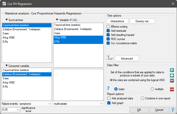
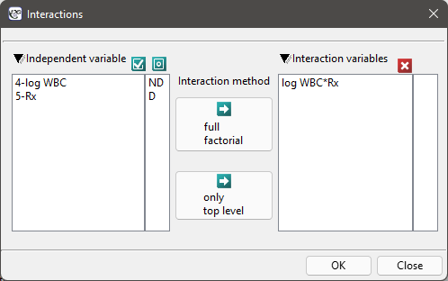
The aim of the study is to determine the influence of kind of treatment on the time of remaining in remission, taking into account possible confounding factors and interactions. In the analysis we will focus on the „Rx (1=placebo, 0=new treatment)” variable. We will place the „log WBC” variable in the model as a possible confounding factor (which modifies the effect). In order to evaluate the possible interactions of „Rx” and „log WBC” we will also consider a third variable, a ratio of the interacting variables. We will add the variable to the model by selecting, in the analysis window, the Interactions button and by setting appropriate options there.

We build three Cox models:

[Model A] only contains the „Rx” variable:

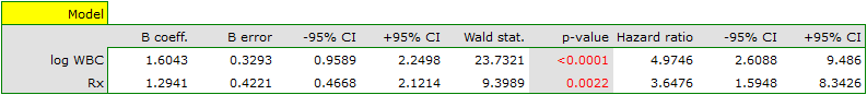
[Model B] contains the „Rx” variable and the potentially confounding variable „log WBC”:

[Model C] ontains the „Rx” variable, the „log WBC” variable, and the potential effect of the interactions of those variables: „Rx $\times$ log WBC”:

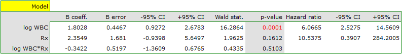
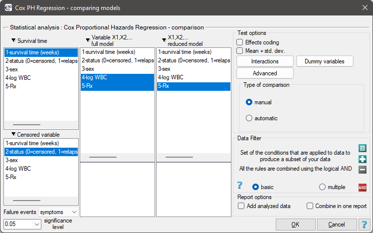
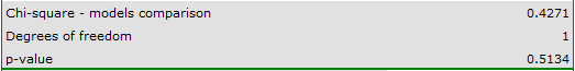
The variable which informs about the interaction of „Rx” and „log WBC”, included in model C, is not significant in model C, according to the Wald test. Thus, we can view further consideration of the interactions of the two variables in the model to be unnecessary. We will obtain similar results by comparing, with the use of a likelihood ratio test, model C with model B. We can make the comparison by choosing the Cox PH regression – comparing models menu. We will then obtain a non-significant result (p=0.5134) which means that model C (model with interaction) is NOT significantly better than model B (model without interaction).

Therefore, we reject model C and move to consider model B and model A.

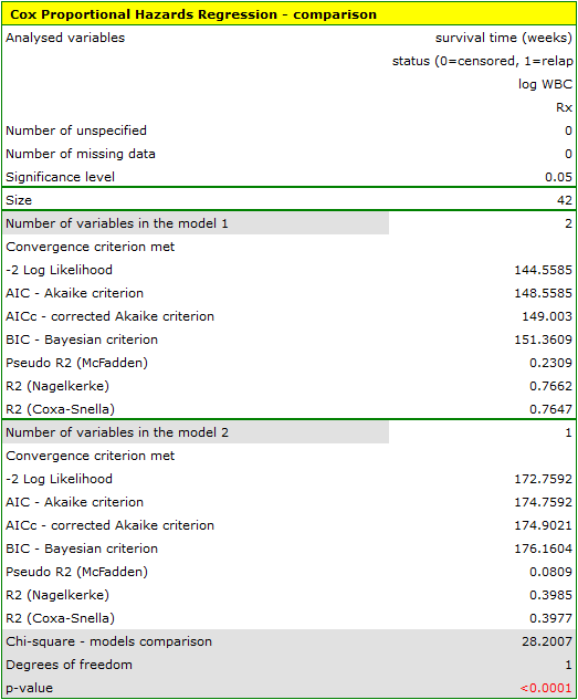
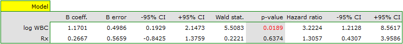
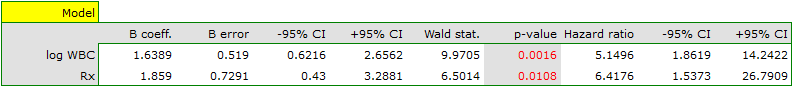
HR for „Rx” in model B is 3.65 which means that hazard for the „placebo group” is about 3.6 greater than for the patients undergoing new treatment. Model A only contains the „Rx” variable, which is why it is usually called a „crude” model – it ignores the effect of potential confounding factors. In that model the HR for „Rx” is 4.52 and is much greater than in model B. However, let us look not only at the point values of the HR estimator but also at the 95\% confidence interval for those estimators. The range for „Rx” in model A is 8.06 (10.09 minus 2.03) wide and is narrower in model B: 6.74 (8.34 minus 1.60). That is why model B gives a more precise HR estimation than model A. In order to make a final decision about which model (A or B) will be better for the evaluation of the effect of treatment („Rx”) we will once more perform a comparative analysis of the models in the Cox PH pregression – comparing models module. This time the likelihood ratio test yields a significant result (p<0.0001), which is the final confirmation of the superiority of model B. 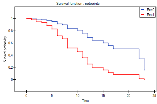That model has the lowest value of information criteria (AIC=148.6, AICc=149 BIC=151.4) and high values of goodness of fit (Pseudo $R^2_{McFadden}=0.2309$ , $R^2_{Nagelkerke}=0.7662$ , $R^2_{Cox-Snell}=0.7647$ ).

The analysis is complemented with the presentation of the survival curves of both groups, the new treatment one and the traditional treatment one, corrected by the influence of „log WBC”, for model B. In the graph we observe the differences between the groups, which occur at particular points of survival time. To plot such curves, after selecting Add Graph, we check the Survival Function: in subgroups ... and then, to quickly build a graph of two curves, I choose Quick subgroups and indicate the variable Rx. The Advanced subgroups option allows you to build any number of arbitrarily defined curves.

At the end we will evaluate the assumptions of Cox regression by analyzing the model residuals with respect to time.

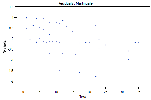
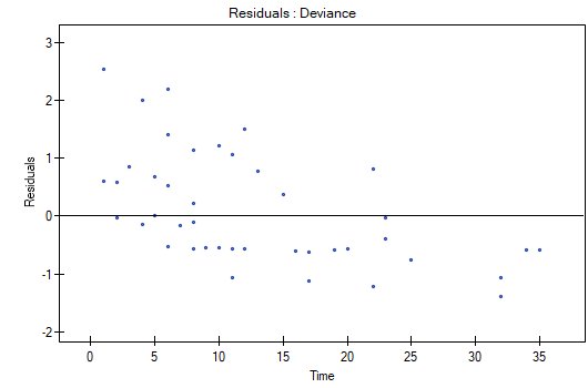
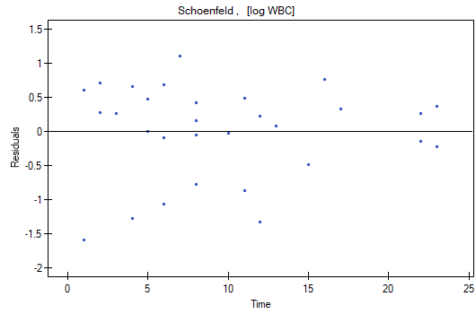
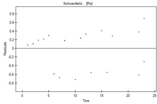
We do not observe any outliers, however, the martingale and deviance residuals become lower the longer the time. Shoenfeld residuals have a symmetrical distribution with respect to time. In their case the analysis of the graph can be supported with various tests which can evaluate if the points of the residual graph are distributed in a certain pattern, e.g. a linear dependency. In order to make such an analysis we have to copy Shoenfeld residuals, together with time, into a datasheet, and test the type of the dependence which we are looking for. The result of such a test for each variable signifies if the assumption of hazard proportionality by a variable in the model has been fulfilled. It has been fulfilled if the result is statistically insignificant and it has not been fulfilled if the result is statistically significant. As a result the variable which does not fulfill the regression assumption of the Cox proportional hazard can be excluded from the model. In the case of the „Log WBC” and „Rx” variables the symmetrical distribution of the residuals suggests the fulfillment of the assumption of hazard proportionality by those variables. That can be confirmed by checking the correlation, e.g. Pearson's linear or Spearman's monotonic, for those residuals and time.

Later we can add the sex variable to the model. However, we have to act with caution because we know, from various sources, that sex can have an influence on the survival function as regards leukemia, in that survival functions can be distributed disproportionately with respect to each other along the time line. That is why we create the Cox model for three variables: „Sex”, „Rx”, and „log WBC”. Before interpreting the coefficients of the model we will check Schonfeld residuals. We will present them in graphs and their results, together with time, will be copied from the report to a new data sheet where we will check the occurrence of Spearman's monotonic correlation. The obtained values are p=0.0259 (for the time and Shoenfeld residuals correlation for sex), p=0.6192 (for the time and Shoenfeld residuals correlation for log WBC), and p=0,1490 (for the time and Shoenfeld residuals correlation for Rx) which confirms that the assumption of hazard proportionality has not been fulfilled by the sex variable. Therefore, we will build the Cox models separately for women and men. For that purpose we will make the analysis twice, with the data filter switched on. First, the filter will point to the female sex (0), second, to the male sex (1).

For women

For men

2022/02/09 12:56

¹⁾

Mantel N. and Haenszel W. (1959), Statistical aspects of the analysis of data from retrospective studies of disease. Journal of the National Cancer Institute, 22,719-748

²⁾

Mantel N. (1966), Evaluation of Survival Data and Two New Rank Order Statistics Arising in Its Consideration. Cancer Chemotherapy Reports, 50:163—170

³⁾ , ⁸⁾

Cox D.R. (1972), Regression models and life tables. Journal of the Royal Statistical Society, B34:187-220

⁴⁾

Gehan E. A. (1965a), A Generalized Wilcoxon Test for Comparing Arbitrarily Singly-Censored Samples. Biometrika, 52:203—223

⁵⁾

Gehan E. A. (1965b), A Generalized Two-Sample Wilcoxon Test for Doubly-Censored Data. Biometrika, 52:650—653

⁶⁾

Tarone R. E., Ware J. (1977), On distribution-free tests for equality of survival distributions. Biometrica, 64(1):156-160

⁷⁾

Armitage P., Berry G., (1994), Statistical Methods in Medical Research (3rd edition); Blackwell

⁹⁾

Breslow N.E. (1974), Covariance analysis of censored survival data. Biometrics, 30(1):89–99

¹⁰⁾

Peduzzi P., Concato J., Feinstein A.R., Holford T.R. (1995), Importance of events per independent variable in proportional hazards regression analysis. II. Accuracy and precision of regression estimates. Journal of Clinical Epidemiology, 48:1503-1510

¹¹⁾

Volinsky C.T., Raftery A.E. (2000) , Bayesian information criterion for censored survival models. Biometrics, 56(1):256–262

¹²⁾

Freireich E.O., Gehan E., Frei E., Schroeder L.R., Wolman I.J., et al. (1963), The effect of 6-mercaptopmine on the duration of steroid induced remission in acute leukemia. Blood, 21: 699–716

¹³⁾

Kleinbaum D. G., Klein M., (2005) Survival Analysis: A Self-Learning Text, Second Edition (Statistics for Biology and Health

PQStat - Baza Wiedzy

Pasek boczny

Spis treści

Survival analysis

Life tables

Kaplan-Meier curves

Comparison of survival curves

Differences among the survival curves

Survival curves trend

Survival curves for the stratas

Cox proportional hazard regression

Hazard Ratio

Model verification

Analysis of model residuals

Comparison of Cox PH regression models

PQStat - Baza Wiedzy

Narzędzia użytkownika

Narzędzia witryny

Pasek boczny

Spis treści

Survival analysis

Life tables

Kaplan-Meier curves

Comparison of survival curves

Differences among the survival curves

Survival curves trend

Survival curves for the stratas

Cox proportional hazard regression

Hazard Ratio

Model verification

Analysis of model residuals

Comparison of Cox PH regression models

Narzędzia strony