Spis treści

Meta-analysis

Meta-analysis

The number of scientific papers being published has increased tremendously in the last decade. This comes with a number of benefits, but it makes it difficult to keep up with the ever-emerging new information. For example, if a doctor were to use a new treatment for his patients based on a scientific paper he had read, he could make a mistake. The error could come from the fact that a whole host of other papers have been published that contradict the effectiveness of that treatment. In order for a doctor's decision to have the least amount of error, he or she should read most of the scientific papers that have been published on the topic. As a result, the constant review of the growing body of literature would take up so much time that there may not be enough time to treat patients. A meta-analysis allows such a review to be done quickly because it is the result of an extensive literature review and a statistical summary of the findings presented therein.

Meta-analysis in PQStat is performed using the following measures:

Mean difference,
d Cohen,
g Hedges,
Ratio of two means,
Odds Ratio (OR),
Relative risk (RR),
Risk difference (RD),
Pearson coefficient,
AUC for ROC curve,
Proportion. .

Introduction

The most familiar image associated with meta-analysis is the forest plot showing the results of each study along with a summary.

$\begin{pspicture}(-2,-0.5)(5,4) \psline{-}(1.4,0)(1.4,4) \psline{->}(0,0)(5,0) \psline[linewidth=0.7pt, linestyle=dotted](2.6,0)(2.6,4) \rput(-0.8,0.8){\scriptsize Summary} \psdiamond[framearc=.3,fillstyle=solid, fillcolor=lightgray](2.6,0.8)(0.4,0.15) \rput(-0.6,1.575){\scriptsize Study 5} \psline[linewidth=0.2pt](2.3,1.575)(2.9,1.575) \psframe[linewidth=0.1pt,framearc=.1,fillstyle=solid, fillcolor=lightgray](2.5,1.5)(2.65,1.65) \rput(-0.6,2.1){\scriptsize Study 4} \psline[linewidth=0.2pt](2.53,2.1)(3.1,2.1) \psframe[linewidth=0.1pt,framearc=.1,fillstyle=solid, fillcolor=lightgray](2.7,2)(2.9,2.2) \rput(-0.6,2.54){\scriptsize Study 3} \psline[linewidth=0.2pt](1,2.54)(3.35,2.54) \psframe[linewidth=0.1pt,framearc=.1,fillstyle=solid, fillcolor=lightgray](2,2.5)(2.08,2.58) \rput(-0.6,3.04){\scriptsize Study 2} \psline[linewidth=0.2pt](1.25,3.04)(3.25,3.04) \psframe[linewidth=0.1pt,framearc=.1,fillstyle=solid, fillcolor=lightgray](2.1,3)(2.18,3.08) \rput(-0.6,3.55){\scriptsize Study 1} \psline[linewidth=0.2pt](0.85,3.55)(2.5,3.55) \psframe[linewidth=0.1pt,framearc=.1,fillstyle=solid, fillcolor=lightgray](1.5,3.5)(1.6,3.6) \rput(2.4,-0.3){\scriptsize Effect size} \end{pspicture}$

In order for the selected literature to be summarized together, it must be consistent in description and the measures given there must be the same.

To be used in a meta-analysis, a scientific paper should describe:

Final result which is some kind of statistical measure indicating the result (effect) obtained in the paper. In fact, these can be different kinds of measures, e.g., difference between means, odds ratio, relative risk, etc.

Standard Error i.e. SE allowing one to determine the precision of the study carried out. This precision assigns the study weight. The smaller the error (SE), the higher the precision of a given study and the higher the assigned weight will be, making a given study more likely to contribute to the results of a meta-analysis.

Group size is the number of objects on which the study was conducted.

Note

It often happens, that a scientific paper does not contain all of the elements listed above, in which case you should look for data in the paper from which the calculation of these measures will be possible.

Note

The PQstat program performs meta-analysis related calculations on data containing: Final Effect, Standard Error, and in some situations Group Size. It is recommended that you enter the data for each publication in the data preparation window before performing the meta-analysis. This is particularly handy when a paper does not explicitly provide these three measures.

The data preparation window is opened via menu: Advanced Statistics→Meta-analysis→Data preparation.

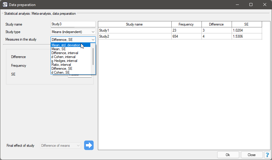
In the data preparation window for meta-analysis, the researcher first provides the name of the study being entered. This name should uniquely identify the study, as it will describe it in all meta-analysis results, including graphs. The desired Final result, Effect Error and Group Size are calculated based on measures extracted from the relevant scientific paper. The measures included in the studies from which the final results can be calculated are shown in the table below:

$\begin{tabular}{|c|c|c|} \hline Study type&Study measures&Final result\\\hline\hline Independent means&Means, st. deviations&\textbf{a}, \textbf{b}, \textbf{c}, \textbf{e}\\ &Means, SE&\textbf{a}, \textbf{b}, \textbf{c}, \textbf{e}\\ &Difference, interval&\textbf{a}\\ &d Cohen, interval&\textbf{b}\\ &g Hadges, interval&\textbf{c}\\ &Ratio, interval&\textbf{e}\\ &Difference, SE&\textbf{a}\\ &d Cohen, SE&\textbf{b}\\ &g Hadges, SE&\textbf{c}\\ &Ratio, SE&e\\\hline Dependent means&Means, st. deviations&\textbf{a}, \textbf{b}, \textbf{c}\\ &Means, SE&\textbf{a}, \textbf{b}, \textbf{c}\\ &Difference, interval&\textbf{a}\\ &d Cohen, interval&\textbf{b}\\ &g Hadges, interval&\textbf{c}\\ &Difference, st. deviation&\textbf{a}, \textbf{b}, \textbf{c}\\ &Difference, SE&\textbf{a}, \textbf{b}, \textbf{c}\\ &d Cohen, SE&\textbf{b}\\ &g Hadges, SE&\textbf{c}\\\hline Mean vs. set&Mean, st. deviation&\textbf{a}\\ &Mean, SE&\textbf{a}\\\hline Mean - summary&Mean, st. deviation&\textbf{d}\\ &Mean, SE&\textbf{d}\\\hline Tables &2x2 Tables&\textbf{b}, \textbf{c}, \textbf{f}, \textbf{g}, \textbf{h}\\ &OR, interval&\textbf{b}, \textbf{c}, \textbf{f}\\ &RR, interval&\textbf{g}\\ &RD, interval&\textbf{h}\\ &d Cohen, interval&\textbf{b}, \textbf{c}, \textbf{f}\\ &g Hadges, interval&\textbf{b}, \textbf{c}, \textbf{f}\\ &OR, SE&\textbf{b}, \textbf{c}, \textbf{f}\\ &RR, SE&\textbf{g}\\ &RD, SE&\textbf{h}\\ &d Cohen, SE&\textbf{b}, \textbf{c}, \textbf{f}\\ &g Hadges, SE&\textbf{b}, \textbf{c}, \textbf{f}\\\hline Correlation&Coefficient&\textbf{i}\\ &Coefficient, interval&\textbf{i}\\ &Coefficient, SE&\textbf{i}\\\hline ROC curve&AUC, SE&\textbf{j}\\ &AUC, interval&\textbf{j}\\\hline One proportion&Set group size&\textbf{k}\\ &Set proportion&\textbf{k}\\\hline \end{tabular}$

where the individual end results are:

a – Difference of means
b – d Cohen
c – g Hadges
d – Mean
e – Ratio of means
f – Odds Ratio (OR)
g – Relative risk (RR)
h – Risk differential (RD)
i – Pearson coefficient
j – AUC (ROC curve)
k – Proportion

Note

In determining the error of coefficients such as OR or RR and others based on tables, when there exist values of zero in the tables or in determining the error of proportions when the proportion is 0 or 1, a continuity correction using an increase factor of 0.5 is applied. The confidence interval for proportions is determined according to the exact Clopper-Pearson method\cite{clopper_pearson}.

EXAMPLE

We are interested in the effect of cigarette smoking on the risk of disease X. We want to conduct a meta-analysis for which the end result will be relative risk (RR). Under this assumption, the papers selected for the meta-analysis must be able to calculate the RR and its error.

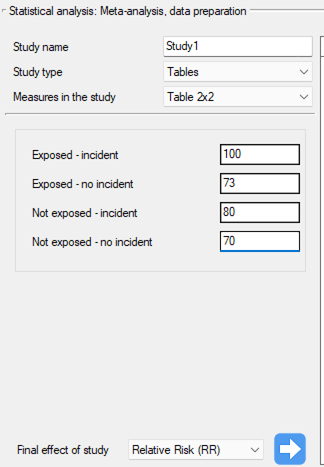
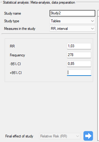
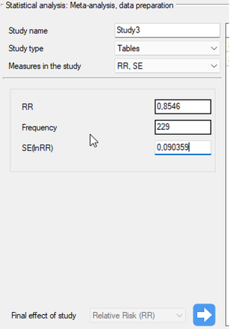
Step 1. Based on the description of the final result (see table above), it was found that the relative risk (described as the score g) is possible to determine in the PQStat program in three situations, i.e., if the RR and the confidence interval for it or the RR together with the error are given in the scientific paper, or if the corresponding group sizes in four categories are given, i.e., a 2×2 table.

Step 2. Ten papers were selected for meta-analysis that met the inclusion criteria and had the potential to determine relative risk (see step 1). The needed data included in the selected papers were:

Study 1: group sizes: (smokers and sick)=100, (smokers and non-sick)=73, (non-smokers and sick)=80, (non-smokers and non-sick)=70,

Study 2: group sizes: (smokers and sick)=182, (smokers and non-sick)=172, (non-smokers and sick)=180, (non-smokers and non-sick)=172,

Study 3: group sizes: (smokers and sick)=157, (smokers and non-sick)=132, (non-smokers and sick)=125, (non-smokers and non-sick)=201,

Study 4: group sizes: (smokers and sick)=19, (smokers and non-sick)=15, (non-smokers and sick)=35, (non-smokers and non-sick)=20,

Study 5: group size: 278, RR[95\%CI]=1.03[0.85-1.25],

Study 6: group size: 560, RR[95\%CI]=1.21[1.05-1.40],

Study 7: group size: 1207, RR[95\%CI]=1.04[0.93-1.15],

Study 8: group size: 214, RR[95\%CI]=1.15[0.95-1.40],

Study 9: group size: 285, RR[95\%CI]=1.36[1.03-1.79],

Study 10: group size: 1968, RR=1.17, SE(lnRR)=0.0437,

Step 3. KUsing the study preparation window for the meta-analysis, data was input into the datasheet. The first four studies are entered by selecting tables, studies five through nine are entered by selecting RR and range, and the last study provides all the necessary data, i.e., RR and SE. We set Relative risk (RR) as the Final effect of the study:

We move each entered study to the window on the right-hand side . Using the OK button, we transfer the prepared studies to the datasheet. Based on the information about each study in the datasheet, you can proceed to perform a meta-analysis.

P-value, and thus statistical significance is not directly used in meta-analysis. The same effect size may be statistically significant in a large study and insignificant in a study based on small sample size. Moreover, a quite small effect size may be statistically significant in a large study, and a quite large effect size may be insignificant in a small study. This fact is related to the power of statistical tests. When testing for statistical significance, we are testing whether an effect exists at all, i.e., whether it is different from zero, not whether it is large enough to translate into desired effects. For example, the fact that a drug statistically significantly lowers blood pressure by 1mmHg will not result in it being used, because 1mmHg is too small from a clinical perspective. Meta-analysis focuses on the magnitude of individual effects rather than their statistical significance. As a result, it does not matter much whether the papers used in the meta-analysis indicate statistical significance of a particular effect or not.

In PQStat, statistical significance is calculated for each study given the effect ratio and the error of that effect. This is an asymptotic approach, based on a normal distribution and dedicated to large samples. If a different test was used to check statistical significance in the cited study, the results obtained may differ slightly.

2022/02/09 12:56

Summary effect

As a result of the meta-analysis, its most desirable element is to summarize the collected studies, i.e., to report the overall effect, $M$ . Such a summary can be done in two ways, by designating a fixed effect or a random effect.

Fixed effect

In calculating the fixed effect, we assume that all studies in the meta-analysis share one common true effect. Thus, if each study involved the same population, e.g., the same country, then to summarize the meta-analysis with a fixed effect we assume that the true (population) effect will be the same in each of these studies. Consequently, all factors that could disturb the size of this effect are the same. For example, if the effect obtained can be affected by the age or gender of the subjects, then these factors are similar in each study. Thus, differences in the obtained effects for individual studies are due only to sampling error (the inherent error of each study) - that is, the size of $SE$ .

The fixed effect estimates the population effect – the true effect for each study.

The confidence interval around the fixed effect (the width of the rhombus in the forest plot) depends only on specific $SE$ .

Random effect

In calculating the random effect, we assume that each study represents a slightly different population, so that the true (population) effect will be different for each population. Thus, if each study involved a different country, then in order to summarize the meta-analysis with a random effect, we assume that some factors that could distort the magnitude of the effect may have different magnitudes across countries. For example, if the effect (e.g., the average increase in fertility) can be affected by the education level of the respondents or the wealth of a country, and these countries differ in these factors, then the true effect (the average increase in fertility) will be slightly different in each of these countries. Thus, the differences in the obtained effects for each study are due to sampling error (the error within each study) – that is, the size of $SE$ , and the differences between the study populations (the variance between the studies - the heterogeneity of the studies) – i.e., $T^2$ . This heterogeneity cannot be too large, too much variance between study populations indicates no basis for a overall summary.

The random effect estimates a weighted mean of the true (population) effects of each study.

The confidence interval around the variable effect (the width of the rhombus in the forest plot) depends on individual $SE$ and on $T^2$ .

Confidence interval vs. prediction interval

95% confidence interval (width of the rhombus in the forest plot) - means that in 95 percent of cases of such meta-analyses the overall random effect will fall into the interval determined by the rhombus.

95% prediction interval - means that 95 percent of the time the true (population) effect of the new study will fall into the designated interval.

The meta-analysis settings window is opened menu: Advanced Statistics→Meta-analysis→Meta-analysis, summary.

In this window, depending on the Final Effect selected, you can summarize the meta-analysis and perform basic analyses to check its assumptions such as heterogeneity, publication bias (sensitivity testing, asymmetry) and perform a cumulative meta-analysis.

EXAMPLE (MetaAnalysisRR.pqs file)

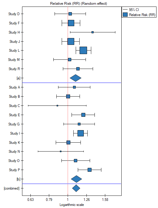
The risk of disease X for smokers and non-smokers has been studied. Some research papers indicated that the risk of disease X was higher for smokers, while some papers did not prove such a relationship. A meta-analysis was planned to determine whether cigarette smoking affects the occurrence of disease X. A thorough review of the literature on this topic was performed, and based on this, 10 scientific papers were selected for meta-analysis. These papers had data on the basis of which it was possible to calculate the relative risk (i.e. the risk of the disease for smokers in relation to the risk of the disease for non-smokers) and it was possible to establish the error with which the given relative risk is burdened (i.e. the precision of the given study). Data were prepared for meta-analysis and stored in a file.

Because the papers included in the meta-analysis were from different locations and included slightly different populations, the summary was chosen using random effect. As the final effect, relative risk was selected and the results were presented on a forest plot.

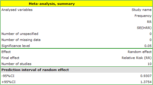
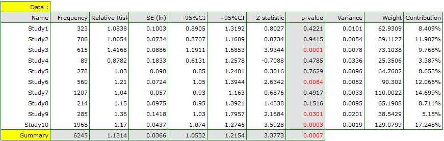
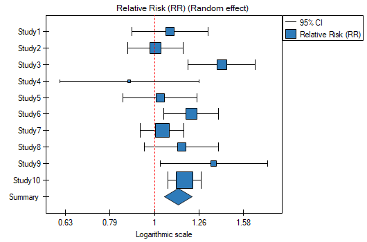
The results of four studies (studies 3, 6, 9, and 10) indicate a significantly higher risk of disease for smokers. The overall result of the meta-analysis conducted is also statistically significant and confirms the same effect. The derived relative risk for the overall effect along with the 95 percent confidence interval is above the value of one: RR[95%CI]=1.13[1.05-1.22]. Unfortunately, the prediction interval for the variable effect is wider: [0.93-1.38], which means that in 95\% of the cases, the true population relative risk obtained in subsequent studies could be either greater or less than one.

Note

Before interpreting the results, it is important to check that the assumptions of the meta-analysis are met. In this case, we should consider excluding the third study (see sensitivity analysis , asymmetry analysis, cumulative meta-analysis and the assumption of heterogeneity).

2022/02/09 12:56

Weights of individual studies

The weight $w_i$ of the study depends on the observed variability.

For the fixed effect, the variability is due only to sampling error (error within each study) - that is, the size of $SE$ :

$\begin{displaymath} w_i=\frac{1}{SE^2} \end{displaymath}$

For a random effect, variability is due to sampling error (error within each study) - that is, the magnitude of $SE$ , and differences between studies – that is, the observed variance $T^2$ :

$\begin{displaymath} w_i=\frac{1}{SE^2+T^2} \end{displaymath}$

Based on the weights assigned to each study, the share of a given study in the entire analysis is determined. This is the percentage that the weight of a given study represents in relation to the total weight of all included studies.

2022/02/09 12:56

Heterogeneity testing

It is difficult to expect every study to end up with exactly the same effect size. Naturally, the results obtained in different papers will be somewhat different. The study of heterogeneity is intended to determine to what extent emerging differences between the results obtained in different papers affect the overall effect constructed in the meta-analysis. The overall effect summarizes well the results obtained in the different papers if the differences between the different effects are natural i.e. not large. Large differences in observed effects may indicate heterogeneity of studies and the need to separate more homogeneous subgroups, e.g., divide the collected papers into several subgroups with respect to an additional factor. For example: a given drug has a different effect on younger and older people, so in studies based on data from mainly young people, the effect may differ significantly from studies conducted on older people. Dividing the collected papers into more homogenous subgroups will allow for a good estimation of the overall effect for each of these subgroups separately.

Heterogeneity testing is designed to check whether the variability between studies is equal to zero.

Hypotheses:

$\begin{array}{cl} \mathcal{H}_0: & \tau^2 = 0,\\ \mathcal{H}_1: & \tau^2 \ne 0, \end{array}$

where:

$\tau^2$ – is the variance of the true (population) effects of each study.

The test statistic is of the form:

$\begin{displaymath} Q=T^2W+k-1 \end{displaymath}$

where:

$T^2$ – is the variance of the observed effects,

$W$ – a factor calculated from the weights assigned to each study,

$k$ – number of studies.

The statistic has asymptotically (for large sample) chi-squared with the degrees of freedom calculated by the formula: $df=k-1$ .

The p value, designated on the basis of the test statistic, is compared with the significance level $\alpha$ :

$\begin{array}{ccl} $ if $ p \le \alpha & \Longrightarrow & $ reject $ \mathcal{H}_0 $ and accept $ \mathcal{H}_1, \\ $ if $ p > \alpha & \Longrightarrow & $ there is no reason to reject $ \mathcal{H}_0. \\ \end{array}$

Note

If the result is statistically significant – this is a strong suggestion to abandon the overall summary of all collected studies.
If the result obtained is not statistically significant – we can summarize the study with the overall effect. At the same time, it is suggested to summarize with a random effect – according to the following explanation.

Rationale for choosing a random effect:

The overall random effect test takes into account the variability between tests ( $T^2$ ), while the fixed overall effect does not take this variability into account. However, if $T^2$ is small, the result of the fixed effect model will be close to that of the random effect model, and when $T^2=0$ , both models will produce exactly the same result. Additional measures describing heterogeneity are the coefficients $I^2$ and $H^2$ :

$\begin{displaymath} I^2=\frac{H^2-1}{H^2},\\ H^2=\frac{Q}{k-1}. \end{displaymath}$

The $I^2$ coefficient indicates the percentage of the observed variance that results from the true difference in the magnitude of the effects under study (graphically, it reflects the extent of overlap between the confidence intervals of the individual studies). Because it falls between 0% and 100%, it is subject to simple interpretation and is readily used. If $I^2=0$ , then all of the observed variance in effect sizes is „ false,” so if a value of 0 is found in the confidence interval drawn around the $I^2$ coefficient, the resulting variance can be considered statistically insignificant. On the other hand, the closer the value of $I^2$ is to 100%, the more one should consider abandoning the overall summary of the study. It is assumed that $I^2\approx 25%$ indicates weak, $I^2\approx 50%$ moderate, and $I^2\approx 75%$ strong heterogeneity among studies. The coefficient $H^2$ , on the other hand, is considered with respect to a value of 1. If the confidence interval for $H^2$ contains a value of 1, then the variance obtained can be considered statistically insignificant, and the higher the value of $H^2$ , the greater the heterogeneity of the study.

EXAMPLE cont (MetaAnalysisRR.pqs file)

When examining the effect of cigarette smoking on the onset of disease X, the heterogeneity assumption of the study was tested. For this purpose, the option Heterogeneity test was selected in the analysis window.

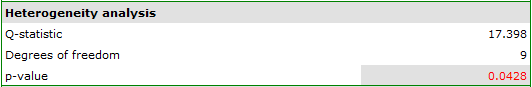
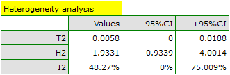
A statistically significant result of Q statistic was obtained (p=0.0428). The variance of the observed effects is non-zero (T2=0.0058), and the coefficient I2=48.27%, indicates moderate heterogeneity between studies. Only the confidence interval for the H2 coefficient finds insignificant variability between studies (the range for this coefficient is [0.93-4.00]). With these results in mind, it is important to consider whether the collected papers can be summarized by one overall result (shared relative risk) or whether it is worthwhile to determine a more homogeneous group of papers and perform the analysis again.

2022/02/09 12:56

Sensitivity testing

The overall effect of a study may change depending on which studies we include and which we exclude from the analysis. It is the responsibility of the researcher to check how sensitive the analysis is to changes in study selection criteria. Checking for sensitivity helps determine the changes in overall effect resulting from removing a particular study. The studies should be close enough that removing one of them does not completely change the interpretation of the overall effect.

The assigned value remaining contribution defines the percentage that the total weight of the remaining studies in the analysis represents when a given study is excluded. In contrast, the precision chenge indicates how the precision of the overall effect (the width of the confidence interval) will change when a given study is excluded from the analysis.

A good illustration of the sensitivity analysis is a forest plot of the effect size and a plot of the change in precision, with each study excluded.

EXAMPLE cont. (MetaAnalysisRR.pqs file)

When examining the effect of cigarette smoking on the onset of disease X, the sensitivity of the analysis was checked to exclude individual studies. To do this, the Sensitivity option was selected in the analysis window and forest plot (sensitivity) and bar plot (sensitivity) were selected..

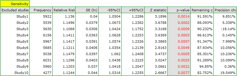
The overall relative risk, however, not including particular, indicated studies, still remain statistically significant. The only caveat is study 3. When it is excluded, the precision of the summary obtained increases. The confidence interval for the overall effect is then narrower by about 18\%.

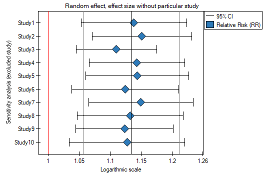
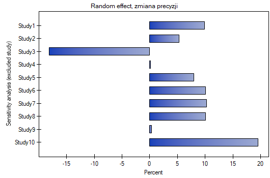
Analysis of the plots leads to the same conclusion. The narrowest interval and the most beneficial change in precision will be obtained when test 3 is excluded.

2022/02/09 12:56

Asymmetry testing

Symmetry in the effects obtained is usually indicative of the absence of publication bias, but it should be kept in mind that many objective factors can disrupt symmetry, e.g., studies with statistically insignificant effects or small studies are often not published, making it much more difficult to reach such results. At the same time, there are no sufficiently comprehensive and universal statistical tools for asymmetry detection. As a result, a significant part of meta-analyses is published despite the diagnosed asymmetry. Such studies, however, require good justification of such a procedure.

Funnel plot

$\begin{pspicture}(-1,-0.5)(7,5) \psline{->}(0,0)(0,4) \psline{->}(0,0)(5,0) \psdots(0.5,0.5) \psdots(1,1) \psdots(1.5,0.5) \psdots(1.5,2) \psdots(1.6,1.1) \psdots(1.8,2.4) \psdots(2,2) \psdots(2,2.8) \psdots(2.1,0.6) \psdots(2.5,4) \psdots(2.5,1.2) \psdots(2.5,2) \psdots(2.5,3) \psdots(2.5,4) \psdots(3,2.6) \psdots(2.8,3.1) \psdots(3,2) \psdots(2,1.3) \psdots(1.5,1.6) \psdots(3.3,2.2) \psellipse[linestyle=dashed,linecolor=red, dash=3pt 2pt](3.5,1)(-0.9,-0.9) \rput(3.5,1){\scriptsize bias} \rput(5.5,1.9){\scriptsize publication bias} \rput(5.9,1.3){\scriptsize asymmetrical plot} \rput(6.5,1.6){\tiny no studies in the bottom right corner of the plot} \end{pspicture}$

A standard way to test for publication bias in the form of asymmetry is a funnel plot, showing the relations between study size (Y axis) and summary effect size (X axis). It is assumed that large studies (placed at the top of the graph) in a correctly selected set, are located close together and define the center of the funnel, while smaller studies are located lower and are more diverse and symmetrically distributed. Instead of the study size on the Y-axis, the effect error for a given study can be shown, which is better than showing the study size alone. This is because the effect error is a measure that indicates the precision of the study and also carries information about its size.

Egger's test

Since the interpretation of a funnel plot is always subjective, it may be helpful to use the Egger coefficient (Egger 1997¹⁾), the interception of the fitted regression line. This coefficient is based on the correlation between the inverse of the standard error and the ratio of the effect size to its error. The further away from 0 the value of the coefficient, the greater the asymmetry. The direction of the coefficient determines the type of asymmetry: a positive value along with a positive confidence interval for it indicates an effect size that is too high in small studies and a negative value along with a negative confidence interval indicates an effect size that is too low in small studies.

Note

Egger's test should only be used when there is a large variation in study sizes and the occurrence of a medium-sized study.

Note

With few studies (small number of $k$ ), it is difficult to reach a significant result despite the apparent asymmetry.

Hypotheses:

$\begin{array}{cl} \mathcal{H}_0: & b = 0,\\ \mathcal{H}_1: & b \ne 0, \end{array}$

where:

$b$ – intercept in Egger's regression equation.

The test statistic is in the form of:

$\begin{displaymath} t=\frac{b}{SE(b)} \end{displaymath}$

where:

$SE(b)$ – standard error of intercept.

The test statistic has t-Student distribution with $k-2$ degrees of freedom.

The p value, designated on the basis of the test statistic, is compared with the significance level $\alpha$ :

$\begin{array}{ccl} $ if $ p \le \alpha & \Longrightarrow & $ reject $ \mathcal{H}_0 $ and accept $ \mathcal{H}_1, \\ $ if $ p > \alpha & \Longrightarrow & $ there is no reason to reject $ \mathcal{H}_0. \\ \end{array}$

Testing the „Fail-safe” number

Rosenthal’s Nfs - The „fail-safe” number described by Rosenthal (1979)²⁾ specifies the number of papers not indicating an effect (e.g., difference in means equal to 0, odds ratio equal to 1, etc.) that is needed to reduce the overall effect from statistically significant to statistically insignificant.

$\begin{displaymath} Nfs=\frac{\left(\sum_{i=1}^{k}Z_i\right)^2}{Z_c^2}-k \end{displaymath}$

where:

$Z_i$ – the value of the test statistic (with normal distribution) of a given test,

$Z_c$ – the critical value of the normal distribution for a given level of significance,

$k$ – number of studies in the meta-analysis.

Rosenthal (1984)³⁾ defined the number of papers being the cutoff point as $5k+10$ . By determining the quotient of $Nfs$ and the cutoff point, we obtain coefficient(fs). According to Rosenthal's interpretation, if coefficient(fs) is greater than 1, the probability of publication bias is minimal.

Orwin's Nfs - the „fail-safe” number described by Orwin (1983) determines the number of papers with the average effect indicated by the researcher $\overline{M_{fs}}$ that is needed to reduce the overall effect to the desired size $M_d$ indicated by the researcher.

$\begin{displaymath} Nfs=k\frac{M - M_d}{M_d-\overline{M_{fs}}} \end{displaymath}$

where:

$M$ – the overall effect obtained in the meta-analysis.

EXAMPLE cont (MetaAnalysisRR.pqs file)

When examining the effect of cigarette smoking on the onset of disease X, the assumption of study asymmetry, and therefore publication bias, was checked. To do this, the option Asymmetry was selected in the analysis window and Funnel plot was selected.

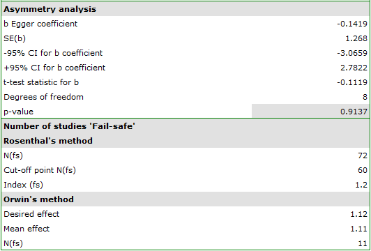
Egger's test result are not statistically significant (p=0.9137), indicating no publication bias.

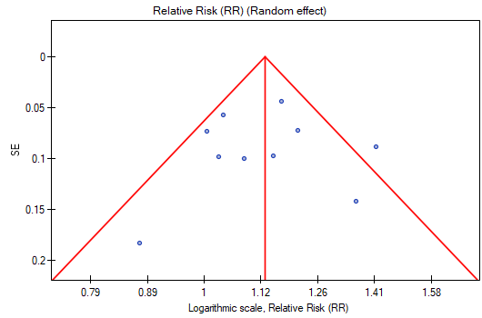
The points representing each study are symmetrically distributed in the funnel plot. Admittedly, one study is outside the boundary of the triangle (Study 3), but it is close to its edges. On the basis of the diagram we also have no fundamental objections to the choice of studies, the only concern being the third study.

The number of „fail-safe” papers determined by Rosenthal's method is large and is at 72. Thus, if the overall effect (relative risk shared by all studies) were to be statistically insignificant (cigarette smoking would have no effect on the risk of disease X), 72 more papers with a relative risk of one would have to be included in the pooled papers. The obtained effect can be therefore considered stable, as it will not be easy (with a small number of papers) to undermine the obtained effect.

The resulting overall relative risk is RR=1.13. Using Orwin's method it was checked how many papers with relative risk equal to 1.11 it would take for the overall relative risk to fall to 1.12. The result was 11 papers. On the other hand, by reducing the size of the relative risk from 1.11 to 1.10 only 5 papers are needed for the overall relative risk to be 1.12.

2022/02/09 12:56

Cumulative meta-analysis

The typical purpose of conducting a cumulative meta-analysis is to show how the effect has changed since the last meta-analysis on a topic was conducted/published, or how it has changed over the years. Then chronologically (according to the timeline) more studies are added and the overall effect is calculated each time. Equally important is the cumulative analysis in a study of how the overall effect changes depending on the magnitude of the impact of a selected additional factor. The studies are then sorted according to the magnitude of that factor and the for successively added studies, a cumulative overall effect is calculated.

Depending on the purpose of the cumulation, the variable by which the individual studies will be sorted should be chosen, i.e., the order in which the studies are added to the meta-analysis summary. This can be any numerical variable.

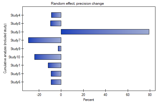
The assigned value of Cumulative contribution defines the percentage that is represented by the total weight of the included studies in the analysis i.e., the given study and the studies preceding it. In contrast, Precision change indicates how the precision of the overall effect (the width of the confidence interval) will change when a given study is included with the studies preceding it.

A good illustration of the cumulative analysis is a forest plot of the effect size and a plot of the change in precision, with each study included.

EXAMPLE cont. (MetaAnalyzisRR.pqs file)

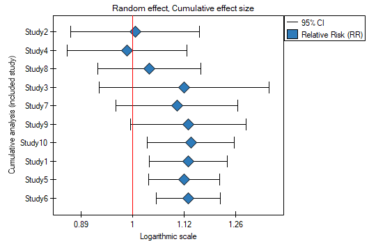
By investigating the effect of cigarette smoking on the onset of disease X, we examined how the results evolved over time. To do this, the cumulative meta-analysis was selected in the analysis window as well as the variable by which subsequent papers would be included in the meta-analysis, and forest plot (cumulative) and bar plot (cumulative) were specified.

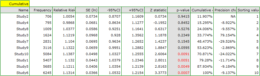
As new papers were added, the resulting overall effect gained strength, and its significance was obtained by adding Study 10 to the earlier papers, and then subsequent studies as well. In general, the addition of more papers increased the precision of the derived relative risk, except when Study 3 was added. The confidence interval of the overall relative risk then increased by 79.15%. We see this effect in the table and in the accompanying charts. As a result, one should consider excluding Study 3 from the meta-analysis.

2022/02/09 12:56

Group comparison

There are situations in which the data collected are of the same effect, performed on the same population, but under slightly different conditions. Suppose that part of the study was performed under condition A and part under condition B. Then it may be interesting to compare the overall effects obtained for each group. Demonstrating differences between overall effects may be the main goal of a meta-analysis, and then it is inadvisable to compound both subgroups simultaneously with one overall effect. However, if the researcher realizes that the studies were conducted under different conditions, but it seems appropriate to summarize all the studies together, then showing the absence of statistically (or clinically) significant differences, the researcher can make a joint summary taking into account this division into subgroups A and B, i.e. determine a overall summary adjusted for different conditions of the experiment. For example, Country A has a slightly different climate than Country B. We have a number of studies from country A and a number of studies from country B. If our study population is the vegetation of these two countries, we can test whether the climatic conditions affect the obtained study effects for each country. A comparative analysis of the subgroups thus determined will allow us to assess whether climate has a major influence on the results obtained or not, and whether the results of the studies covering these two countries can indeed be summarized in one overall effect, or whether we should determine separate summaries for each country. Another example can be a situation where some of the studies are studies in which randomization was performed, but in some of them we do not have full randomization, then we can divide the studies into subgroups to then check whether the studies without randomization give similar results to the studies with randomization in order to include them in further, combined analysis.

Group heterogeneity

Examination of group heterogeneity

We can compare groups by choosing as overall effect: fixed effect, random effect – separate $T^2$ or random effect – pooled $T^2$ , where $T^2$ is the variance of the observed effects.

Fixed effect is chosen when we assume that studies within each group share one common true (i.e., population) effect.
Random effect (separate $T^2$ ) is chosen when we assume that the studies within each group represent slightly different populations, and the groups differ in variance between studies.
Random effect (pooled $T^2$ ) is chosen when we assume that the studies within each group represent slightly different populations, but the variance between studies is the same, regardless of the group to which they belong.

The main goal is to compare groups, that is, to determine whether the groups being compared differ in their true (i.e., population) overall effect. In practice, this is to test whether the variance of group overall effects is zero, i.e., to test the heterogeneity of the groups. For a description and interpretation of the results of heterogeneity analysis, see chapter Heterogeneity testing, except that in the case of group comparisons, heterogeneity refers to the compound effects of the groups being compared, not the individual studies, and the outcome depends on the overall effect chosen.

Hypotheses:

$\begin{array}{cl} \mathcal{H}_0: & \tau^2 = 0,\\ \mathcal{H}_1: & \tau^2 \ne 0, \end{array}$

where:

$\tau^2$ – is the variance of the true (population) summary effects of the groups being compared.

The p value, designated on the basis of the test statistic, is compared with the significance level $\alpha$ :

$\begin{array}{ccl} $ if $ p \le \alpha & \Longrightarrow & $ reject $ \mathcal{H}_0 $ and accept $ \mathcal{H}_1, \\ $ if $ p > \alpha & \Longrightarrow & $ there is no reason to reject $ \mathcal{H}_0. \\ \end{array}$

If the result is statistically significant (a score of Q-statistic, $I^2$ coefficient or $H^2$ coefficient), this is a strong suggestion to drop the overall summary of the groups being compared.

Examining heterogeneity in groups

An additional option of the analysis is the possibility to analyze each group separately for heterogeneity, as described in Heterogeneity testing. The results obtained (in particular, the variance $T^2$ ) make it easier to decide how to compare the groups, i.e., whether to choose a random effect (separate $T^2$ ) or a random effect (pooled $T^2$ ).

Joint summary of the groups

In a situation where, based on the results of the group comparison, the differences obtained between the overall effects of the groups are small and insignificant, a joint summary of the groups can be performed. The summation is done in correction for the division into the indicated groups. For example, if we split the study based on the different conditions of the experiment conducted, then the joint summary will be done in correction for the different conditions of the experiment. The result of joint summation (overall efect of both grous) depends on the observed differences (on the variation between studies and between groups) i.e. on the choice of ovearall effect (whether it is fixed or random (separate $T^2$ ) or random (pooled $T^2$ )).

A good illustration of the joint (ovearall) summary of the groups in the meta-analysis is a forest plot showing the results of each study with each group's summary and the joint summary of the groups.

ANOVA comparison

ANOVA comparison is an additional option for comparing groups. It is a slightly different method of comparison than comparison by testing heterogeneity of groups (based on a different mathematical model). Both methods, however, give overlapping results as to the comparison of groups. In case of comparison of groups by ANOVA method the observed variance is broken down into between-group variance and within-group variance. The within-group variance is then broken down into the variance of each group separately. As a result, the following $Q$ statistics are determined:

The $Q$ statistic (group 1) – examines that part of the total variance that relates to group one, i.e., the variance between studies located within group one,
The $Q$ statistic (group 2) – examines that part of the total variance that relates to the second group, i.e. the variance between studies within the second group,
…
The $Q$ statistic (group g) – examines that part of the total variance that relates to the last group, i.e., the variance between studies within the last group,
The $Q$ statistic (within groups) = $Q$ (group 1) + $Q$ (group 2) + … + $Q$ (group g) - examines that part of the total variance that relates to the inside of the individual groups, i.e., the variance of the within-group tests,
The $Q$ statistic (between groups) - examines that part of the total variance that relates to differences between groups, i.e., the between-group variance (same result as examining the heterogeneity of groups) ,
The $Q$ statistic (total) - examines the variance between all studies.

Each of the above $Q$ statistics has a chi-square distribution with the appropriate number of degrees of freedom.

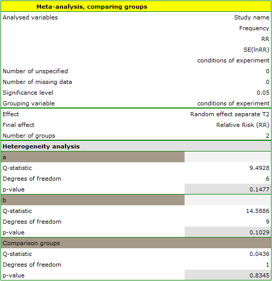
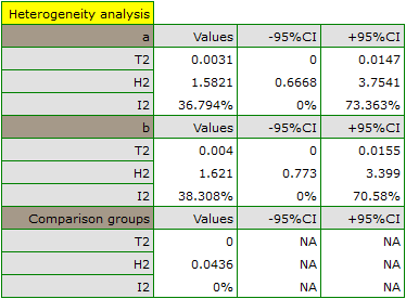
The window with settings of group comparison for meta-analysis is opened via menu: Advanced Statistics→Meta-analysis→Meta-analysis, comparing groups.

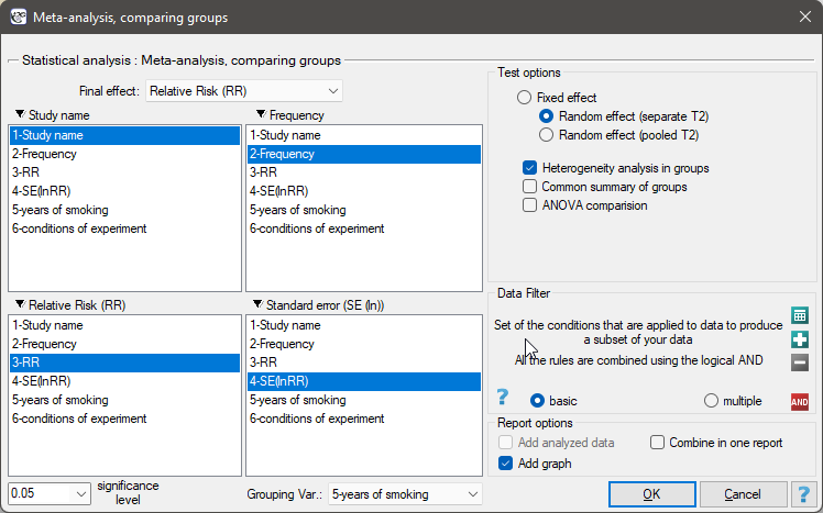
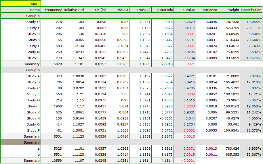
EXAMPLE (MetaAnalysisRR.pqs file)

The risk of disease X was examined for smokers and non-smokers. A meta-analysis was conducted to determine whether smoking duration affects the onset of disease X. A thorough review of the literature on this topic was carried out, and 17 studies were identified that had a description of the relative risk and its error (i.e. the precision of the study). Because the studies involved different smoking times, 3 groups of studies were identified:

(1) studies on people who have been smoking for more than 10 years,

(2) studies on people who have been smoking for 5 to 10 years,

(3) studies on people who have been smoking for less than 5 years.

In addition, a subdivision was made between the two different conditions of the studies (different inclusion/exclusion criteria of subjects). Data were prepared for meta-analysis and stored in a file.

The purpose of conducting the meta-analysis was to compare age groups. In addition, it was examined whether the different conditions of the experiment translated into differences in the relative risk obtained.

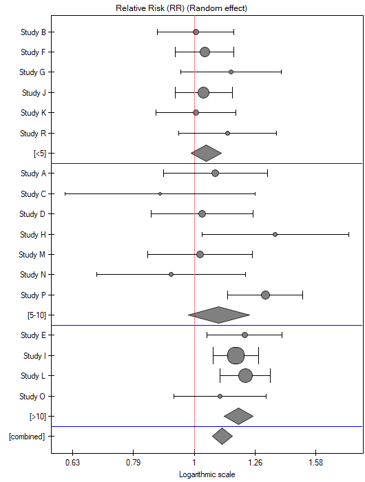
Because the papers included in the meta-analysis were from different locations and included slightly different populations, the summary was made by selecting random effect (separate T2). As the final effect, relative risk was selected and the results were presented on a forest plot.

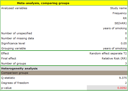
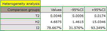
The groups are statistically significantly different (p=0.0092), which we observe not only based on the test of heterogeneity, but also on the coefficient of H2 (the coefficient along with the confidence interval is above the value of one) and I2 (78 is high heterogeneity). Therefore, the collected papers will not be summarized by a overall effect but only by a separate summary of each group.

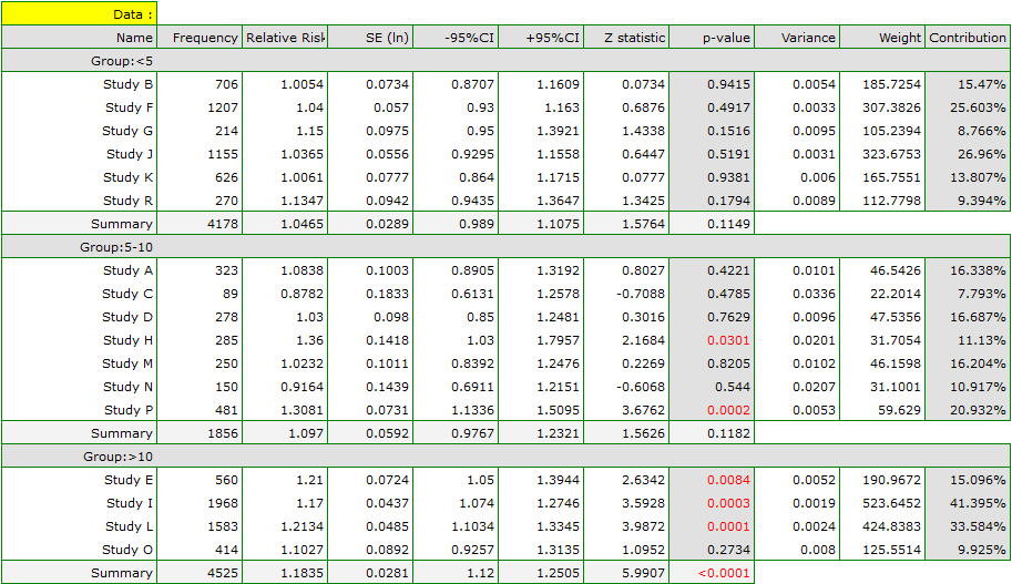
The forest plot also shows a summary of each group and does not contain a joint summary of the groups.

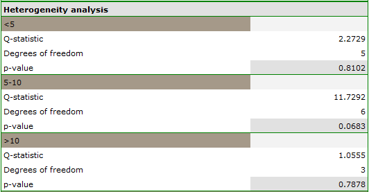
In addition, homogeneity within each group was checked to ascertain the feasibility of summarizing them separately.

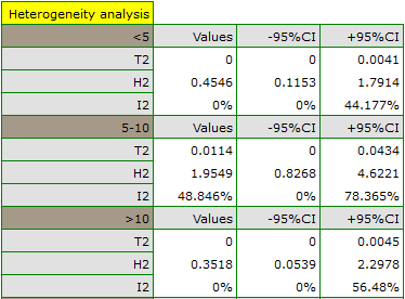
In contrast, the results of the comparison concerning the different study conditions indicate that there is no significant effect of these conditions on the overall effect. In this case, it is possible to calculate a joint overall effect when correcting for the different test conditions, i.e., a joint summary of the two groups.

2022/02/09 12:56

Meta-regression

Meta-regression analysis is conducted in an analogous manner to the regression analysis described in the section Multiple Regression. In the case of meta-regression, the study objects are the individual studies, their results (e.g., odds ratios, relative risks, differences in means) constitute the dependent variable $Y$ i.e., the explained variable, and the additional conditions for conducting these studies constitute the independent variables ( $X_1$ , $X_2$ , $\ldots$ , $X_k$ ) i.e., the explanatory variables. As in traditional regression models, the independent variables may interact and those described by a nominal scale may be subject to special coding (for more information, see Preparation of the variables for analysis in multivariate models). The number of independent variables should be small, less than the number of papers on which the study is based on ( $n\ge k+1$ ).

We can perform meta-regression by choosing a fixed effect or a random effect.

Fixed effect is chosen when we assume that the studies represent one common true effect such that all factors that could perturb the magnitude of this effect are the same except for the factors tested as independent variables in the model ( $X_1$ , $X_2$ , $\ldots$ , $X_k$ ). This is a situation that occurs very rarely in real research because it requires fully controlled conditions, which is almost impossible in different studies, conducted in different locations and by different researchers. The use of fixed effect would be justified, for example, in a situation when all the tests are carried out at the same location, on the same population, changing only those conditions that are described by the characteristic being tested. For example, if we wanted to test the effect of changing temperature on changing the relative risk of disease described in each study, then all studies should be conducted on the same population under exactly the same conditions except for the change in temperature, which is the independent variable $X$ in the model.
Random effect is chosen when we assume that studies may represent slightly different populations, i.e., factors that could perturb the magnitude of the effect under study are not described in all papers (they can be assumed to be similar, but not necessarily exactly the same). Each paper provides the magnitudes of the factors we are interested in, which are involved in model building as independent variables ( $X_1$ , $X_2$ , $\ldots$ , $X_k$ ). The use of a random effect is common because individual studies are usually conducted at different locations under slightly different conditions, the variability of interest is only in the conditions that describe the factors given in the study, e.g., temperature, which will be the independent variable $X$ in the model.

Model verification

Statistical significance of individual variables in the model.

Based on the coefficient and its error, we can conclude whether the independent variable for which this coefficient was estimated has a significant effect on the final effect. For this purpose, we test the hypotheses:

$\begin{array}{cc} \mathcal{H}_0: & \beta_i=0,\\ \mathcal{H}_1: & \beta_i\ne 0. \end{array}$

Calculate the test statistic using the formula:

$\begin{displaymath} Z=\frac{b_i}{SE_{b_i}} \end{displaymath}$

Test statistics has the normal distribution.

The p value, designated on the basis of the test statistic, is compared with the significance level $\alpha$ :

$\begin{array}{ccl} $ if $ p \le \alpha & \Longrightarrow & $ reject $ \mathcal{H}_0 $ and accept $ \mathcal{H}_1, \\ $ if $ p > \alpha & \Longrightarrow & $ there is no reason to reject $ \mathcal{H}_0. \\ \end{array}$

Quality of the built model of a linear multivariate regression can be assessed by several measures.

Coefficient $R^2$ – is a measure of model fit. It expresses the percentage of variability between study effects explained by the model.

The value of this coefficient is in the range $<0; 1>$ , where 1 means a perfect fit of the model, 0 – a complete lack of fit. In determining it we use the following equation:

$\begin{displaymath} R^2=T^2_{(modelu)}+T^2_{(total)}, \end{displaymath}$

where:

$T^2_{(modelu)}$ – variance between studies explained by the model,

$T^2_{(total)}$ – total variance between studies.

Coefficient $I^2$ – determines the percentage of the observed variance that results from the true difference in the magnitude of the effects under study.

Note

For a detailed representation of the variance described by the coefficients, see chapter Testing heterogeneity

Statistical significance of all variables in the model

The primary tool for estimating the significance of all variables in the model is an ANOVA that determines $Q$ (of the model).

$\begin{array}{cc} \mathcal{H}_0: & \textrm{all } \beta_i=0,\\ \mathcal{H}_1: & \textrm{exists }\beta_i\neq0. \end{array}$

Using the ANOVA approach, the observed variance between tests is broken into the variance explained by the model and the variance of the residual (not explained by the model). As a result, the following $Q$ statistics are determined:

The $Q$ statistic (of the residuals) - examines the portion of the total variance that is not explained by the model,
The $Q$ statistic (of the model) - examines the portion of the total variance that is explained by the model,
The $Q$ statistic (total) - examines the variance between all studies.

Each of the above $Q$ statistics has chi-square distribution with the appropriate number of degrees of freedom.

The p value, designated on the basis of the test statistic, is compared with the significance level $\alpha$ :

$\begin{array}{ccl} $ if $ p \le \alpha & \Longrightarrow & $ reject $ \mathcal{H}_0 $ and accept $ \mathcal{H}_1, \\ $ if $ p > \alpha & \Longrightarrow & $ there is no reason to reject $ \mathcal{H}_0. \\ \end{array}$

The window with settings of group comparison for meta-analysis is opened via menu: Advanced Statistics→Meta-analysis→Meta-regression.

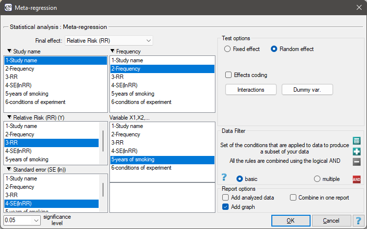
EXAMPLE cont. (MetaAnalysisRR.pqs file)

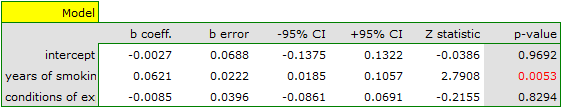
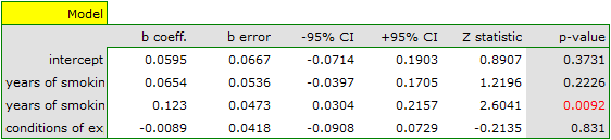
The risk of disease X was examined for smokers and non-smokers. A meta-analysis comparing groups of studies was conducted to determine whether the number of years of smoking affected the onset of disease X and whether different conditions of the experiment resulted in different relative risks. On the basis of the comparison of the groups of studies, it was possible to establish that the last group (the group of smokers who have been smoking the longest, i.e. for more than 10 years) shows an association between smoking and the onset of disease X. On the other hand, for the groups with shorter smoking duration, no significant effect could be obtained. However, it was observed that the effect systematically increased with increasing years of smoking. To test the hypothesis of a significant increase in the risk of disease X with increasing years of smoking, two regression models were constructed. In the first model, the grouping variable Years of smoking was treated as a continuous variable. In the second model, it was determined that the variable Years of smoking would be treated as a categorical (dummy) variable with the reference group smoking less than 5 years. Data were prepared for meta-regression and stored in a file.

Because the papers included in the meta-analysis were from different locations and included slightly different populations, the meta-regression was performed by selecting random effect. The relative risk was selected as the final effect, and the results were presented in the graph.

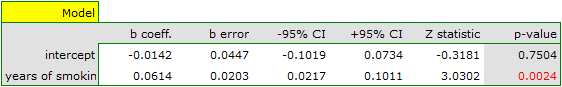
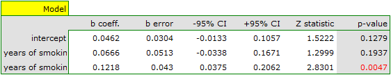
Both models confirmed a significant association between the duration of smoking and the magnitude of the relative risk of disease X. In the first model, the logarithm of the relative risk of disease X increased by 0.0614 with increasing time of smoking (moving to the subsequent group of years of smoking). Analysis of the results of the second model leads to similar conclusions. In this case, the results are considered for the group of smokers smoking less than 5 years. The logarithm of relative risk for smokers between 5 and 10 years increases by 0.0666 (relative to smokers younger than 5 years), and for smokers older than 10 years it increases by 0.1218 (relative to smokers younger than 5 years).

Since part of the study was conducted according to other criteria (under different conditions) the obtained results of both models were corrected for different conditions of the study.

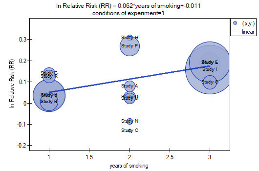
The correction performed did not change the underlying trend, and thus it can be concluded that the risk of disease X increases with years of smoking regardless of what methodology (inclusion/exclusion criteria of subjects) was used to conduct the study. The resulting relation for the first model, assuming that the study was conducted under condition „a” (indicated as first conditions) is shown in the graph.

2022/02/09 12:56

¹⁾

Egger M., Smith G. D., Schneider M., Minder C (1997), Bias in meta-analysis detected by a simple, graphical test. BMJ, 315(7109):629-634

²⁾

Rosenthal R. (1979), The „file drawer problem” and tolerance for null results. Psychological Bulletin, 5, 638-641

³⁾

Orwin R. G. (1983), A Fail-SafeN for Effect Size in Meta-Analysis. J Educ Behav Stat, 8(2):157-159

PQStat - Baza Wiedzy

Pasek boczny

Spis treści

Meta-analysis

Introduction

Summary effect

Weights of individual studies

Heterogeneity testing

Sensitivity testing

Asymmetry testing

Cumulative meta-analysis

Group comparison

Group heterogeneity

Meta-regression

Model verification

PQStat - Baza Wiedzy

Narzędzia użytkownika

Narzędzia witryny

Pasek boczny

Spis treści

Meta-analysis

Introduction

Summary effect

Weights of individual studies

Heterogeneity testing

Sensitivity testing

Asymmetry testing

Cumulative meta-analysis

Group comparison

Group heterogeneity

Meta-regression

Model verification

Narzędzia strony