Multidimensional models

Multivariate regression models provide an opportunity to study the effects of multiple independent variables (multiple factors) and their interactions on a single dependent variable. Through multivariate models, it is also possible to build many simplified models at the same time - one-dimensional (univariate) models. The information about which model we want to build (multivariate or univariate) is visible in the window of the selected analysis. When multiple independent variables are simultaneously selected in the analysis window, it is possible to choose the model.

Preparation of variables for analysis

Matching groups

Why is group matching done?

There are many answers to this question. Let us use an example of a medical situation.

If we estimate the treatment effect from a fully randomized experiment, then by randomly assigning subjects to the treated and untreated groups we create groups that are similar in terms of possible confounding factors. The similarity of the groups is due to the random assignment itself. In such studies, we can examine the pure (not dependent on confounding factors) effect of the treatment method on the outcome of the experiment. In this case, other than random group matching is not necessary.

The possibility of error arises when the difference in treatment outcome between treated and untreated groups may be due not to the treatment itself, but to a factor that induced people to take part in the treatment. This occurs when randomization is not possible for some reason, such as it is an observational study or for ethical reasons we cannot assign treatment arbitrarily. Artificial group matching may then be applicable. For example, if the people we assign to the treatment group are healthier people and the people who are in the control group are people with more severe disease, then it is not the treatment itself but the condition of the patient before treatment that may affect the outcome of the experiment. When we see such an imbalance of groups, it is good if we can decide to randomize, in this way the probem is solved, because drawing people into groups makes them similar. However, we can imagine another situation. This time the group we are interested in will not be treatment subjects but smokers, and the control group will be non-smokers, and the analyses will aim to show the adverse effect of smoking on the occurrence of lung cancer. Then, in order to test whether smoking does indeed increase the risk of lung cancer, it would be unethical to perform a fully randomized trial because it would mean that people randomly selected to the risk group would be forced to smoke. The solution to this situation is to establish an exposure group, i.e. to select a number of people who already smoke and then to select a control group of non-smokers. The control group should be selected because by leaving the selection to chance we may get a non-smoking group that is younger than the smokers only due to the fact that smoking is becoming less fashionable in our country, so automatically there are many young people among the non-smokers.The control should be drawn from non-smokers, but so that it is as similar as possible to the treatment group.In this way we are getting closer to examining the pure (independent of selected confounding factors such as age) effect of smoking/non-smoking on the outcome of the experiment, which in this case is the occurrence of lung cancer. Such a selection can be made by the matching proposed in the program.

One of the main advantages of investigator-controlled matching is that the control group becomes more similar to the treatment group, but this is also the biggest disadvantage of this method. It is an advantage because our study is looking more and more like a randomized study. In a randomized trial, the treatment and control groups are similar on almost all characteristics, including those we don't study - the random allocation provides us with this similarity. With investigator-controlled matching, the treatment and control groups become similar on only selected characteristics.

Ways of assessing similarity:

The first two methods mentioned are based on matching groups through Propensity Score Matching, PSM. This type of matching was proposed by Rosenbaum and Rubin ¹⁾. In practice, it is a technique for matching a control group (untreated or minimally/standardly treated subjects) to a treatment group on the basis of a probability describing the subjects' propensity to assign treatment depending on the observed associated variables. The probability score describing propensity, called the Propensity Score is a balancing score, so that as a result of matching the control group to the treatment group, the distribution of measured associated variables becomes more similar between treated and untreated subjects. The third method does not determine the probability for each individual, but determines a distance/dissimilarity matrix that indicates the objects that are closest/most similar in terms of multiple selected characteristics.

Methods for determining similarity:

Known probability – the Propensity Score, which is a value between 0 and 1 for each person tested, indicates the probability of being in the treatment group. This probability can be determined beforehand by various methods. For example, in a logistic regression model, through neural networks, or many other methods. If a person in the group from which we draw controls obtains a Propensity Score similar to that obtained by a person in the treatment group, then that person can enter the analysis because the two are similar in terms of the characteristics that were considered in determining the Propensity Score.
Calculated from the logistic regression model – because logistic regression is the most commonly used matching method, PQStat provides the ability to determine a Propensity Score value based on this method automatically in the analysis window. The matching proceeds further using the Propensity Score thus obtained.
Similarity/distance matrix – This option does not determine the value of Propensity Score, but builds a matrix indicating the distance of each person in the treatment group to the person in the control group. The user can set the boundary conditions, e.g. he can indicate that the person matched to a person from the treatment group cannot differ from him by more than 3 years of age and must be of the same sex. Distances in the constructed matrix are determined based on any metric or method describing dissimilarity. This method of matching the control group to the treated group is very flexible. In addition to the arbitrary choice of how the distances/dissimilarity are determined, in many metrics it allows for the indication of weights that determine how important each variable is to the researcher, i.e., the similarity of some variables may be more important to the researcher while the similarity of others is less important. However, great caution is advised when choosing a distance/ dissimilarity matrix. Many features and many sops to determine distances require prior standardization or normalization of the data, moreover, choosing the inverse of distance or similarity (rather than dissimilarity) may result in finding the most distant and dissimilar objects, whereas we normally use these methods to find similar objects. If the researcher does not have specific reasons for changing the metric, the standard recommendation is to use statistical distance, i.e. the Mahalanobia metric – It is the most universal, does not require prior standardization of data and is resistant to correlation of variables. More detailed description of distances and dissimilarity/similarity measures available in the program as well as the method of inetrpratation of the obtained results can be found in the Similarity matrix section .

In practice, there are many methods to indicate how close the objects being compared are, in this case treated and untreated individuals. Two are proposed in the program:

Nearest neighbor method – is a standard way of selecting objects not only with a similar Propensity Score, but also those whose distance/dissimilarity in the matrix is the smallest.
The nearest neighbor method, closer than… – works in the same way as the nearest neighbor method, with the difference that only objects that are close enough can be matched. The limit of this closeness is determined by giving a value describing the threshold, behind which there are already objects so dissimilar to the tested objects, that we do not want to give them a chance to join the newly built control group. In the case when analysis is based on Propensity Score or matrix defined by dissimilarity, the most dissimilar objects are those distant by 1, and the most similar are those distant by 0. Choosing this method we should give a value closer to 0, when we select more restrictively, or closer to 1, when the threshold will be placed further. When we determine distances instead of dissimilarities in the matrix, then the minimum size is also 0, but the maximum size is not predetermined.

We can match without returning already drawn objects or with returning these objects again to the group from which we draw.

Matching without returning – when using no-return matching, once an untreated person has been selected for matching with a given treated person, that untreated person is no longer available for consideration as a potential match for subsequent treated persons. As a result, each untreated individual is included in at most one matching set.
Matching with returning – return matching allows a given untreated individual to be included more than once in a single matched set. When return matching is used, further analyses, and in particular variance estimation, must take into account the fact that the same untreated individual may be in multiple matched sets.

In the case when it is impossible to match the untreated person to the treated one, because in the group from which we choose there are more persons matching the treated one equally well, then one of these persons chosen in a random way is combined. For a renewed analysis, a fixed seed is set by default so that the results of a repeated draw will be the same, but when the analysis is performed again the seed is changed and the result of the draw may be different.

If it is not possible to match an untreated person to a treated one, because there are no more persons to join in the group from which we are choosing, e.g. matching persons have already been joined to other treated persons or the set from which we are choosing has no similar persons, then this person remains without a pair.

Most often a 1:1 match is made,i.e., for one treated person, one untreated person is matched. However, if the original control group from which we draw is large enough and we need to draw more individuals, then we can choose to match 1:k, where k indicates the number of individuals that should be matched to each treated individual.

Matching evaluation

After matching the control group to the treatment group, the results of such matching can be returned to the worksheet, i.e. a new control group can be obtained. However, we should not assume that by applying the matching we will always obtain satisfactory results. In many situations, the group from which we draw does not have a sufficient number of such objects that are sufficiently similar to the treatment group. Therefore, the matching performed should always be evaluated. There are many methods of evaluating the matching of groups. The program uses methods based on standardized group difference and Propensity Score percentile agreement of the treatment group and the control group, more extensively described in the work of P.C Austin, among others ²⁾³⁾. This approach allows comparison of the relative balance of variables measured in different units, and the result is not affected by sample size. The estimation of concordance using statistical tests was abandoned because the matched control group is usually much smaller than the original control group, so that the obtained p-values of tests comparing the test group to the smaller control group are more likely to be left with the null hypothesis, and therefore do not show significant differences due to the reduced size.

For comparison of continuous variables we determine the standardized mean difference:

$\begin{displaymath} d=\frac{\left(\bar{x}_{treated}-\bar{x}_{control}\right)}{\sqrt{\frac{sd^2_{treated}+sd^2_{control}}{2}}} \end{displaymath}$

where:

$\bar{x}_{treated}$ , $\bar{x}_{control}$ – is the mean value of the variable in the treatment group and the mean value of the variable in the control group,

$sd^2_{treated}$ , $sd^2_{control}$ – is the variance in the treatment group and the variance in the control group.

To compare binary variables (of two categories, usually 0 and 1) we determine the standardized frequency difference:

$\begin{displaymath} d=\frac{\left(\hat{p}_{treated}-\hat{p}_{control}\right)}{\sqrt{\frac{\hat{p}_{treated}(1-\hat{p}_{treated})+\hat{p}_{control}(1-\hat{p}_{control})}{2}}} \end{displaymath}$

where:

$\hat{p}_{treated}$ , $\hat{p}_{control}$ – is the frequency of the value described as 1 in the treatment group and the frequency of the value described as 1 in the control group.

Variables with multiple categories we should break down in logistic regression analysis into dummy variables with two categories and, by checking the fits of both groups, determine the standardized frequency difference for them.

Note

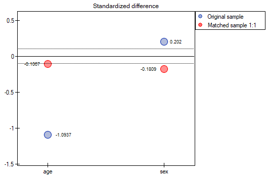
Although there is no universally agreed criterion for what threshold of standardized difference can be used to indicate significant imbalance, a standardized difference of less than 0.1 (in both mean and frequency estimation) can provide a clue ⁴⁾. Therefore, to conclude that the groups are well matched, we should observe standardized differences close to 0, and preferably not outside the range of -0.1 to 0.1. Graphically, these results are presented in a dot plot. Negative differences indicate lower means/frequencies in the treatment group, positive in the control group.

Note

The 1:1 match obtained in the reports means the summary for the study group and the corresponding control group obtained in the first match, the 1:2 match means the summary for the study group and the corresponding control group obtained in the first + second match (i.e., not the study group and the corresponding control group obtained in the second match only), etc.

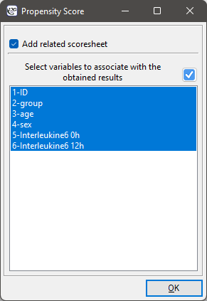
The window with the settings of group matching options is launched from the menu Advanced statistics→Multivariate models→Propensity Score

EXAMPLE (matching.pqs file)

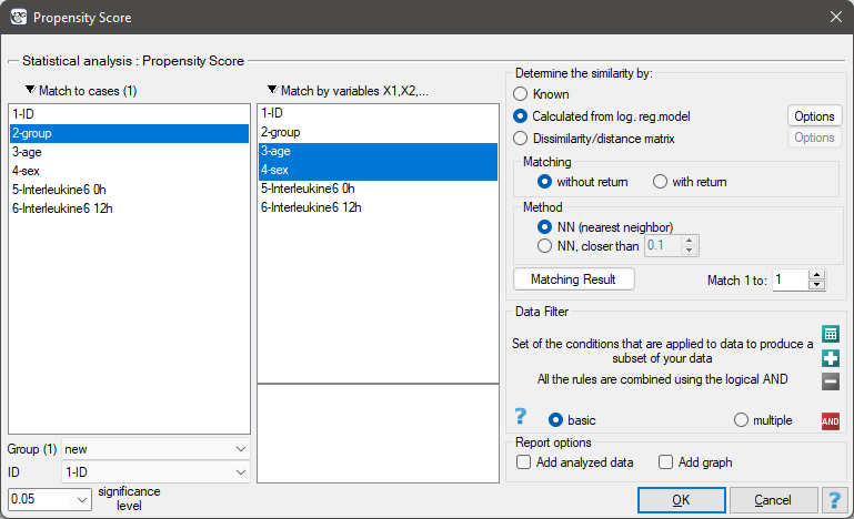
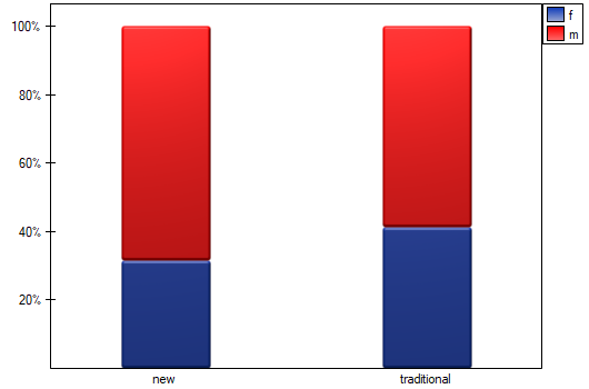
We want to compare two ways of treating patients after accidents, the traditional way and the new one. The correct effect of both treatments should be observed in the decreasing levels of selected cytokines. To compare the effectiveness of the two treatments, they should both be carried out on patients who are quite similar. Then we will be sure that any differences in the effectiveness of these treatments will be due to the treatment effect itself and not to other differences between patients assigned to different groups. The study is a posteriori, that is, it is based on data collected from patients' treatment histories. Therefore, the researchers had no influence on the assignment of patients to the new drug treatment group and the traditional treatment group. It was noted that the traditional treatment was mainly prescribed to older patients, while the new treatment was prescribed to younger patients, in whom it is easier to lower cytokine levels. The groups were fairly similar in gender structure, but not identical.

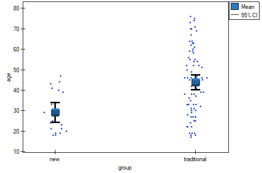
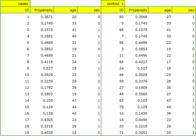
If the planned study had been carried out on such selected groups of patients, the new way would have had an easier challenge, because younger organisms might have responded better to the treatment. The conditions of the experiment would not be equal for both ways, which could falsify the results of the analyses and the conclusions drawn. Therefore, it was decided to match the group treated traditionally to be similar to the study group treated with the new way. We planned to make the matching with respect to two characteristics, i.e. age and gender. The traditional treatment group is larger (80 patients) than the new treatment group (19 patients), so there is a good chance that the groups will be similar. Random selection is performed by the logistic regression model algorithm embedded in the PSM. We remember that gender should be coded numerically, since only numerical values are involved in the logistic regression analysis. We choose nearest neighbor as the method. We want the same person to be unable to be selected duplicately, so we choose a no return randomization. We will try 1:1 matching, i.e. for each person treated with the new drug we will match one person treated traditionally. Remember that the matching is random, so it depends on the random value of seed set by our computer, so the randomization performed by the reader may differ from the values presented here.

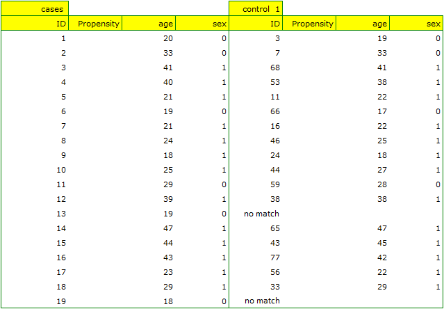
A summary of the selection can be seen in the tables and charts.

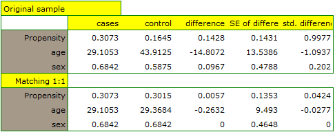
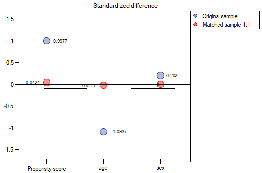
The line at 0 indicates equilibrium of the groups (difference between groups equal to 0). When the groups are in equilibrium with respect to the given characteristics, then all points on the graph are close to this line, i.e., around the interval -0.1 to 0.1. In the case of the original sample (blue color), we see a significant departure of Propensity Score. As we know, this mismatch is mainly due to age mismatch – its standardized difference is at a large distance from 0, and to a lesser extent gender mismatch.

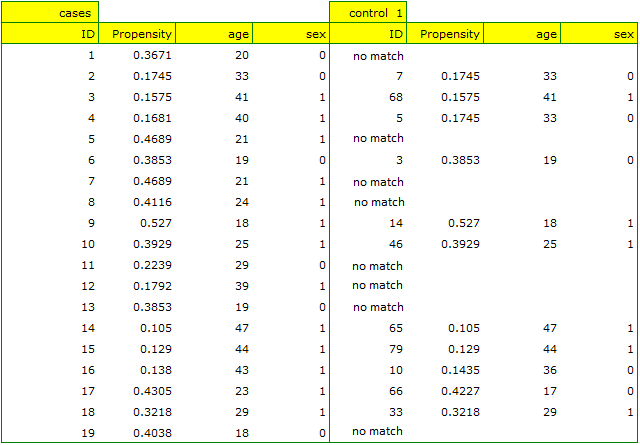
By performing the matching we obtained groups more similar to each other (red color in the graph). The standardized difference between the groups as determined by Propensity Score is 0.0424, which is within the specified range. The age of both groups is already similar – the traditional treatment group differs from the new treatment group by less than a year on average (the difference between the averages presented in the table is 0.2632) and the standardized difference between the averages is -0.0277. In the case of gender, the match is perfect, i.e. the percentage of females and males is the same in both groups (the standardized difference between the percentages presented in the table and the graph is now 0). We can return the data prepared in this way to the worksheet and subject it to the analyses we have planned.

Looking at the summary we just obtained, we can see that despite the good balancing of the groups and the perfect match of many individuals, there are individuals who are not as similar as we might expect.

Sometimes in addition to obtaining well-balanced groups, researchers are interested in determining the exact way of selecting individuals, i.e. obtaining a greater influence on the similarity of objects as to the value of Propensity Score or on the similarity of objects as to the value of specific characteristics. Then, if the group from which we draw is sufficiently large, the analysis may yield results that are more favorable from the researcher's point of view, but if in the group from which we draw there is a lack of objects meeting our criteria, then for some people we will not be able to find a match that meets our conditions.

Suppose that we would like to obtain such groups whose Propensity Score (i.e., propensity to take the survey) differs by no more than …

How to determine this value? You can take a look at the report from the earlier analysis, where the smallest and largest distance between the drawn objects is given.

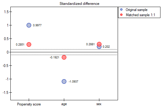
In our case the objects closest to each other differ by min=0, and the furthest by max=0.5183. We will try to check what kind of selection we will obtain when we will match to people treated with the new method such people treated traditionally, whose Propensity Score will be very close to e.g. less than 0.01.

We can see that this time with failed to select the whole group. Comparing Propensity Score for each pair (treated with the new method and treated traditionally) we can see that the differences are really small. However, since the matched group is much smaller, to sum up the whole process we have to notice that both Propensity Score, age and sex are not close enough to the line at 0. Our will to improve the situation did not lead to the desired effect, and the obtained groups are not well balanced.

Suppose we wanted to obtain such pairs (subjects treated with the new method and subjects treated traditionally) who are of the same sex and whose ages do not differ by more than 3 years. In the Propensity Score-based randomization, we did not have this type of ability to influence the extent of concordance of each variable. For this we will use a different method, not based on Propensity Score, but based on distance/dissimilarity matrices. After selecting the Options button, we select the proposed Mahalanobis statistical distance matrix and set the neighborhood fit to a maximum distance equal to 3 for age and equal to 0 for gender. As a result, for two people we failed to find a match, but the remaining matches meet the set criteria.

To summarize the overall draw, we note that although it meets our assumptions, the resulting groups are not as well balanced as they were in our first draw based on Propensity Score. The points in red representing the quality of the match by age and the quality of the match by gender deviate slightly from the line of sameness set at level 0, which means that the average difference in age and sex structure is now greater than in the first matching.

It is up to the researcher to decide which way of preparing the data will be more beneficial to them.

Finally, when the decision is made, the data can be returned to a new worksheet. To do this, go back to the report you selected and in the project tree under the right button select the Redo analysis menu. In the same analysis window, point to the Fit Result button and specify which other variables will be returned to the new worksheet.

This will result in a new data sheet with side-by-side data for people treated with the new treatment and matched people treated traditionally.

2022/02/26 15:35 · admin

Interctions

Interactions are considered in multidimensional models. Their presence means that the influence of the independent variable ( $X_1$ ) on the dependent variable ( $Y$ ) differs depending on the level of another independent variable ( $X_2$ ) or a series of other independent variables. To discuss the interactions in multidimensional models one must determine the variables informing about possible interactions, i.e the product of appropriate variables. For that purpose we select the Interactions button in the window of the selected multidimensional analysis. In the window of interactions settings, with the CTRL button pressed, we determine the variables which are to form interactions and transfer the variables into the neighboring list with the use of an arrow. By pressing the OK button we will obtain appropriate columns in the datasheet.

In the analysis of the interaction the choice of appropriate coding of dichotomous variables allows the avoidance of the over-parametrization related to interactions. Over-parametrization causes the effects of the lower order for dichotomous variables to be redundant with respect to the confounding interactions of the higher order. As a result, the inclusion of the interactions of the higher order in the model annuls the effect of the interactions of the lower orders, not allowing an appropriate evaluation of the latter. In order to avoid the over-parametrization in a model in which there are interactions of dichotomous variables it is recommended to choose the option effect coding.

In models with interactions, remember to „trim” them appropriately, so that when removing the main effects, we also remove the effects of higher orders that depend on them. That is: if in a model we have the following variables (main effects): $X_1$ , $X_2$ , $X_3$ and interactions: $X_1*X_2$ , $X_1*X_3$ , $X_2*X_3$ , $X_1*X_2*X_3$ , then by removing the variable $X_1$ from the model we must also remove the interactions in which it occurs, viz: $X_1*X_2$ , $X_1*X_3$ and $X_1*X_2*X_3$ .

2022/02/09 12:56

Variables coding

When preparing data for a multidimensional analysis there is the problem of appropriate coding of nominal and ordinal variables. That is an important element of preparing data for analysis as it is a key factor in the interpretation of the coefficients of a model. The nominal or ordinal variables divide the analyzed objects into two or more categories. The dichotomous variables (in two categories, $k=2$ ) must only be appropriately coded, whereas the variables with many categories ( $k>2$ ) ought to be divided into dummy variables with two categories and coded.

[ $k=2$ ] If a variable is dichotomous, it is the decision of the researcher how the data representing the variable will be entered, so any numerical codes can be entered, e.g. 0 and 1. In the program one can change one's coding into effect coding by selecting that option in the window of the selected multidimensional analysis. Such coding causes a replacement of the smaller value with value -1 and of the greater value with value 1.
[ $k>2$ ] If a variable has many categories then in the window of the selected multidimensional analysis we select the button Dummy variables and set the reference/base category for those variables which we want to break into dummy variables. The variables will be dummy coded unless the effect coding option will be selected in the window of the analysis – in such a case, they will be coded as -1, 0, and 1.

Dummy coding is employed in order to answer, with the use of multidimensional models, the question: How do the ( $Y$ ) results in any analyzed category differ from the results of the reference category. The coding consists in ascribing value 0 or 1 to each category of the given variable. The category coded as 0 is, then, the reference category.

[ $k=2$ ] If the coded variable is dichotomous, then by placing it in a regression model we will obtain the coefficient calculated for it, ( $b_i$ ). The coefficient is the reference of the value of the dependent variable $Y$ for category 1 to the reference category (corrected with the remaining variables in the model).
[ $k>2$ ] If the analyzed variable has more than two categories, then $k$ categories are represented by $k-1$ dummy variables with dummy coding. When creating variables with dummy coding one selects a category for which no dummy category is created. That category is treated as a reference category (as the value of each variable coded in the dummy coding is equal to 0.

When the $X_1, X_2, ..., X_{k-1}$ variables obtained in that way, with dummy coding, are placed in a regression model, then their $b_1, b_2, ..., b_{k-1}$ coefficients will be calculated.

[ $b_1$ ] is the reference of the $Y$ results (for codes 1 in $X_1$ ) to the reference category (corrected with the remaining variables in the model);
[ $b_2$ ] is the reference of the $Y$ results (for codes 1 in $X_2$ ) to the reference category (corrected with the remaining variables in the model);
[…]
[ $b_{k-1}$ ] is the reference of the $Y$ results (for codes 1 in $X_{k-1}$ ) to the reference category (corrected with the remaining variables in the model);

Example

We code, in accordance with dummy coding, the sex variable with two categories (the male sex will be selected as the reference category), and the education variable with 4 categories (elementary education will be selected as the reference category).

$\mbox{\begin{tabular}{|c|c|} \hline &\textcolor[rgb]{0.5,0,0.5}{\textbf{Coded}}\\ \textbf{Sex}&\textcolor[rgb]{0.5,0,0.5}{\textbf{sex}}\\\hline f&\textcolor[rgb]{0.5,0,0.5}{1}\\ f&\textcolor[rgb]{0.5,0,0.5}{1}\\ f&\textcolor[rgb]{0.5,0,0.5}{1}\\ \cellcolor[rgb]{0.88,0.88,0.88}m&\cellcolor[rgb]{0.88,0.88,0.88}0\\ \cellcolor[rgb]{0.88,0.88,0.88}m&\cellcolor[rgb]{0.88,0.88,0.88}0\\ f&\textcolor[rgb]{0.5,0,0.5}{1}\\ f&\textcolor[rgb]{0.5,0,0.5}{1}\\ \cellcolor[rgb]{0.88,0.88,0.88}m&\cellcolor[rgb]{0.88,0.88,0.88}0\\ \cellcolor[rgb]{0.88,0.88,0.88}m&\cellcolor[rgb]{0.88,0.88,0.88}0\\ f&\textcolor[rgb]{0.5,0,0.5}{1}\\ \cellcolor[rgb]{0.88,0.88,0.88}m&\cellcolor[rgb]{0.88,0.88,0.88}0\\ f&\textcolor[rgb]{0.5,0,0.5}{1}\\ \cellcolor[rgb]{0.88,0.88,0.88}m&\cellcolor[rgb]{0.88,0.88,0.88}0\\ f&\textcolor[rgb]{0.5,0,0.5}{1}\\ \cellcolor[rgb]{0.88,0.88,0.88}m&\cellcolor[rgb]{0.88,0.88,0.88}0\\ \cellcolor[rgb]{0.88,0.88,0.88}m&\cellcolor[rgb]{0.88,0.88,0.88}0\\ ...&...\\\hline \end{tabular}$

$\mbox{\begin{tabular}{|c|ccc|} \hline & \multicolumn{3}{c|}{\textbf{Coded education}}\\ \textbf{Education}&\textcolor[rgb]{0,0,1}{\textbf{vocational}}&\textcolor[rgb]{1,0,0}{\textbf{secondary}}&\textcolor[rgb]{0,0.58,0}{\textbf{tertiary}}\\\hline \cellcolor[rgb]{0.88,0.88,0.88}elementary&\cellcolor[rgb]{0.88,0.88,0.88}0&\cellcolor[rgb]{0.88,0.88,0.88}0&\cellcolor[rgb]{0.88,0.88,0.88}0\\ \cellcolor[rgb]{0.88,0.88,0.88}elementary&\cellcolor[rgb]{0.88,0.88,0.88}0&\cellcolor[rgb]{0.88,0.88,0.88}0&\cellcolor[rgb]{0.88,0.88,0.88}0\\ \cellcolor[rgb]{0.88,0.88,0.88}elementary&\cellcolor[rgb]{0.88,0.88,0.88}0&\cellcolor[rgb]{0.88,0.88,0.88}0&\cellcolor[rgb]{0.88,0.88,0.88}0\\ \textcolor[rgb]{0,0,1}{vocational}&\textcolor[rgb]{0,0,1}{1}&0&0\\ \textcolor[rgb]{0,0,1}{vocational}&\textcolor[rgb]{0,0,1}{1}&0&0\\ \textcolor[rgb]{0,0,1}{vocational}&\textcolor[rgb]{0,0,1}{1}&0&0\\ \textcolor[rgb]{0,0,1}{vocational}&\textcolor[rgb]{0,0,1}{1}&0&0\\ \textcolor[rgb]{1,0,0}{secondary}&0&\textcolor[rgb]{1,0,0}{1}&0\\ \textcolor[rgb]{1,0,0}{secondary}&0&\textcolor[rgb]{1,0,0}{1}&0\\ \textcolor[rgb]{1,0,0}{secondary}&0&\textcolor[rgb]{1,0,0}{1}&0\\ \textcolor[rgb]{1,0,0}{secondary}&0&\textcolor[rgb]{1,0,0}{1}&0\\ \textcolor[rgb]{0,0.58,0}{tertiary}&0&0&\textcolor[rgb]{0,0.58,0}{1}\\ \textcolor[rgb]{0,0.58,0}{tertiary}&0&0&\textcolor[rgb]{0,0.58,0}{1}\\ \textcolor[rgb]{0,0.58,0}{tertiary}&0&0&\textcolor[rgb]{0,0.58,0}{1}\\\ \textcolor[rgb]{0,0.58,0}{tertiary}&0&0&\textcolor[rgb]{0,0.58,0}{1}\\ \textcolor[rgb]{0,0.58,0}{tertiary}&0&0&\textcolor[rgb]{0,0.58,0}{1}\\ ...&...&...&...\\\hline \end{tabular}$

Building on the basis of dummy variables, in a multiple regression model, we might want to check what impact the variables have on a dependent variable, e.g. $Y$ = the amount of earnings (in thousands of PLN). As a result of such an analysis we will obtain sample coefficients for each dummy variable:

- for sex the statistically significant coefficient $b_{i}=-0.5$ , which means that average women's wages are a half of a thousand PLN lower than men's wages, assuming that all other variables in the model remain unchanged;

- for vocational education the statistically significant coefficient $b_{i}=0.6$ , which means that the average wages of people with elementary education are 0.6 of a thousand PLN higher than those of people with elementary education, assuming that all other variables in the model remain unchanged;

- for secondary education the statistically significant coefficient $b_{i}=1$ , which means that the average wages of people with secondary education are a thousand PLN higher than those of people with elementary education, assuming that all other variables in the model remain unchanged;

- for tertiary-level education the statistically significant coefficient $b_{i}=1.5$ , which means that the average wages of people with tertiary-level education are 1.5 PLN higher than those of people with elementary education, assuming that all other variables in the model remain unchanged;

Effect coding is used to answer, with the use of multidimensional models, the question: How do ( $Y$ ) results in each analyzed category differ from the results of the (unweighted) mean obtained from the sample. The coding consists in ascribing value -1 or 1 to each category of the given variable. The category coded as -1 is then the base category

[ $k=2$ ] If the coded variable is dichotomous, then by placing it in a regression model we will obtain the coefficient calculated for it, ( $b_i$ ). The coefficient is the reference of $Y$ for category 1 to the unweighted general mean (corrected with the remaining variables in the model).
If the analyzed variable has more than two categories, then $k$ categories are represented by $k-1$ dummy variables with effect coding. When creating variables with effect coding a category is selected for which no separate variable is made. The category is treated in the models as a base category (as in each variable made by effect coding it has values -1).

When the $X_1, X_2, ..., X_{k-1}$ variables obtained in that way, with effect coding, are placed in a regression model, then their $b_1, b_2, ..., b_{k-1}$ coefficients will be calculated.

[ $b_1$ ] is the reference of the $Y$ results (for codes 1 in $X_1$ ) to the unweighted general mean (corrected by the remaining variables in the model);
[ $b_2$ ] is the reference of the $Y$ results (for codes 1 in $X_2$ ) to the unweighted general mean (corrected by the remaining variables in the model);
[…]
[ $b_{k-1}$ ] is the reference of the $Y$ results (for codes 1 in $X_{k-1}$ ) to the unweighted general mean (corrected by the remaining variables in the model);

Example

With the use of effect coding we will code the sex variable with two categories (the male category will be the base category) and a variable informing about the region of residence in the analyzed country. 5 regions were selected: northern, southern, eastern, western, and central. The central region will be the base one.

$\mbox{\begin{tabular}{|c|c|} \hline &\textcolor[rgb]{0.5,0,0.5}{\textbf{Coded}}\\ \textbf{Sex}&\textcolor[rgb]{0.5,0,0.5}{\textbf{sex}}\\\hline f&\textcolor[rgb]{0.5,0,0.5}{1}\\ f&\textcolor[rgb]{0.5,0,0.5}{1}\\ f&\textcolor[rgb]{0.5,0,0.5}{1}\\ \cellcolor[rgb]{0.88,0.88,0.88}m&\cellcolor[rgb]{0.88,0.88,0.88}-1\\ \cellcolor[rgb]{0.88,0.88,0.88}m&\cellcolor[rgb]{0.88,0.88,0.88}-1\\ f&\textcolor[rgb]{0.5,0,0.5}{1}\\ f&\textcolor[rgb]{0.5,0,0.5}{1}\\ \cellcolor[rgb]{0.88,0.88,0.88}m&\cellcolor[rgb]{0.88,0.88,0.88}-1\\ \cellcolor[rgb]{0.88,0.88,0.88}m&\cellcolor[rgb]{0.88,0.88,0.88}-1\\ f&\textcolor[rgb]{0.5,0,0.5}{1}\\ \cellcolor[rgb]{0.88,0.88,0.88}m&\cellcolor[rgb]{0.88,0.88,0.88}-1\\ f&\textcolor[rgb]{0.5,0,0.5}{1}\\ \cellcolor[rgb]{0.88,0.88,0.88}m&\cellcolor[rgb]{0.88,0.88,0.88}-1\\ f&\textcolor[rgb]{0.5,0,0.5}{1}\\ \cellcolor[rgb]{0.88,0.88,0.88}m&\cellcolor[rgb]{0.88,0.88,0.88}-1\\ \cellcolor[rgb]{0.88,0.88,0.88}m&\cellcolor[rgb]{0.88,0.88,0.88}-1\\ ...&...\\\hline \end{tabular}$

$\mbox{\begin{tabular}{|c|cccc|} \hline \textbf{Regions}& \multicolumn{4}{c|}{\textbf{Coded regions}}\\ \textbf{of residence}&\textcolor[rgb]{0,0,1}{\textbf{western}}&\textcolor[rgb]{1,0,0}{\textbf{eastern}}&\textcolor[rgb]{0,0.58,0}{\textbf{northern}}&\textcolor[rgb]{0.55,0,0}{\textbf{southern}}\\\hline \cellcolor[rgb]{0.88,0.88,0.88}central&\cellcolor[rgb]{0.88,0.88,0.88}-1&\cellcolor[rgb]{0.88,0.88,0.88}-1&\cellcolor[rgb]{0.88,0.88,0.88}-1&\cellcolor[rgb]{0.88,0.88,0.88}-1\\ \cellcolor[rgb]{0.88,0.88,0.88}central&\cellcolor[rgb]{0.88,0.88,0.88}-1&\cellcolor[rgb]{0.88,0.88,0.88}-1&\cellcolor[rgb]{0.88,0.88,0.88}-1&\cellcolor[rgb]{0.88,0.88,0.88}-1\\ \cellcolor[rgb]{0.88,0.88,0.88}central&\cellcolor[rgb]{0.88,0.88,0.88}-1&\cellcolor[rgb]{0.88,0.88,0.88}-1&\cellcolor[rgb]{0.88,0.88,0.88}-1&\cellcolor[rgb]{0.88,0.88,0.88}-1\\ \textcolor[rgb]{0,0,1}{western}&\textcolor[rgb]{0,0,1}{1}&0&0&0\\ \textcolor[rgb]{0,0,1}{western}&\textcolor[rgb]{0,0,1}{1}&0&0&0\\ \textcolor[rgb]{0,0,1}{western}&\textcolor[rgb]{0,0,1}{1}&0&0&0\\ \textcolor[rgb]{0,0,1}{western}&\textcolor[rgb]{0,0,1}{1}&0&0&0\\ \textcolor[rgb]{1,0,0}{eastern}&0&\textcolor[rgb]{1,0,0}{1}&0&0\\ \textcolor[rgb]{1,0,0}{eastern}&0&\textcolor[rgb]{1,0,0}{1}&0&0\\ \textcolor[rgb]{1,0,0}{eastern}&0&\textcolor[rgb]{1,0,0}{1}&0&0\\ \textcolor[rgb]{1,0,0}{eastern}&0&\textcolor[rgb]{1,0,0}{1}&0&0\\ \textcolor[rgb]{0,0.58,0}{northern}&0&0&\textcolor[rgb]{0,0.58,0}{1}&0\\ \textcolor[rgb]{0,0.58,0}{northern}&0&0&\textcolor[rgb]{0,0.58,0}{1}&0\\ \textcolor[rgb]{0.55,0,0}{southern}&0&0&0&\textcolor[rgb]{0.55,0,0}{1}\\ \textcolor[rgb]{0.55,0,0}{southern}&0&0&0&\textcolor[rgb]{0.55,0,0}{1}\\ \textcolor[rgb]{0.55,0,0}{southern}&0&0&0&\textcolor[rgb]{0.55,0,0}{1}\\ ...&...&...&...&...\\\hline \end{tabular}$

Building on the basis of dummy variables, in a multiple regression model, we might want to check what impact the variables have on a dependent variable, e.g. $Y$ = the amount of earnings (expressed in thousands of PLN). As a result of such an analysis we will obtain sample coefficients for each dummy variable:

- for sex the statistically significant coefficient $b_{i}=-0.5$ , which means that the average women's wages are a half of a thousand PLN lower than the average wages in the country, assuming that the other variables in the model remain unchanged;

- for the western region the statistically significant coefficient $b_{i}=0.6$ , which means that the average wages of people living in the western region of the country are 0.6 thousand PLN higher than the average wages in the country, assuming that the other variables in the model remain unchanged;

- for the eastern region the statistically significant coefficient $b_{i}=-1$ , which means that the average wages of people living in the eastern region of the country are a thousand PLN lower than the average wages in the country, assuming that the other variables in the model remain unchanged;

- for the northern region the statistically significant coefficient $b_{i}=0.4$ , which means that the average wages of people living in the western region of the country are 0.4 thousand PLN higher than the average wages in the country, assuming that the other variables in the model remain unchanged;

- for the southern region the statistically significant coefficient $b_{i}=0.1$ , which means that the average wages of people living in the southern region of the country do not differ in a statistically significant manner from the average wages in the country, assuming that the other variables in the model remain unchanged;

2022/02/09 12:56

Multiple Linear Regression

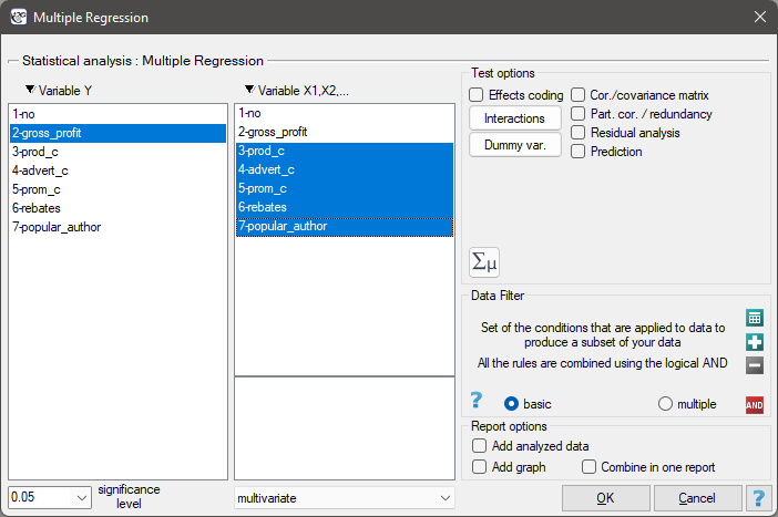
The window with settings for Multiple Regression is accessed via the menu Advanced statistics→Multidimensional Models→Multiple Regression

The constructed model of linear regression allows the study of the influence of many independent variables( $X_1,X_2,\ldots,X_k$ ) on one dependent variable( $Y$ ). The most frequently used variety of multiple regression is Multiple Linear Regression. It is an extension of linear regression models based on Pearson's linear correlation coefficient. It presumes the existence of a linear relation between the studied variables. The linear model of multiple regression has the form: $\begin{displaymath} Y=\beta_0+\beta_1X_1+\beta_2X_2+\ldots+\beta_kX_k+\epsilon. \end{displaymath}$

where:

$Y$ - dependent variable, explained by the model,

$X_1,X_2,\ldots X_k$ - independent variables, explanatory,

$\beta_0,\beta_1,\beta_2,\ldots \beta_k$ - parameters,

$\epsilon$ - random parameter (model residual).

If the model was created on the basis of a data sample of size $n$ the above equation can be presented in the form of a matrix: $\begin{displaymath} Y=X\beta+\epsilon. \end{displaymath}$

where:

$Y=\left( \begin{array}{ccc} y_1\\ y_2\\ \vdots\\ y_n \end{array} \right),$

$X=\left( \begin{array}{ccccc} 1 & x_{11} & x_{21} & \ldots & x_{k1}\\ 1 & x_{12} & x_{22} & \ldots & x_{k2}\\ \vdots & \vdots & \vdots & \ddots & \vdots\\ 1 & x_{1n} & x_{2n} & \ldots & x_{kn} \end{array}\right),$

$\beta=\left( \begin{array}{ccc} \beta_0\\ \beta_1\\ \beta_2\\ \vdots\\ \beta_k \end{array} \right),$

$\epsilon=\left(\begin{array}{ccc} \epsilon_1\\ \epsilon_2\\ \vdots\\ \epsilon_n \end{array} \right).$

In such a case, the solution of the equation is the vector of the estimates of parameters $\beta_0,\beta_1,\ldots,\beta_k$ called regression coefficients:

$b=\left( \begin{array}{ccc} b_0\\ b_1\\ b_2\\ \vdots\\ b_k \end{array} \right).$

Those coefficients are estimated with the help of the classical least squares method. On the basis of those values we can infer the magnitude of the effect of the independent variable (for which the coefficient was estimated) on the dependent variable. They inform by how many units will the dependent variable change when the independent variable is changed by 1 unit. There is a certain error of estimation for each coefficient. The magnitude of that error is estimated from the following formula:

$\begin{displaymath} SE_b=\sqrt{\frac{1}{n-(k+1)}e^Te(X^TX)^{-1}}, \end{displaymath}$

where:

$e=Y-\widehat{Y}$ is the vector of model residuals (the difference between the actual values of the dependent variable Y and the values $\widehat{Y}$ predicted on the basis of the model).

Dummy variables and interactions in the model

A discussion of the coding of dummy variables and interactions is presented in chapter Preparation of the variables for the analysis in multidimensional models.

Note When constructing the model one should remember that the number of observations should meet the assumptions ( $n\ge 50 +8k$ ) where $k$ is the number of explanatory variables in the model ⁵⁾.

Model verification

Statistical significance of particular variables in the model.

On the basis of the coefficient and its error of estimation we can infer if the independent variable for which the coefficient was estimated has a significant effect on the dependent variable. For that purpose we use t-test.

Hypotheses:

$\begin{array}{cc} \mathcal{H}_0: & \beta_i=0,\\ \mathcal{H}_1: & \beta_i\ne 0. \end{array}$

Let us estimate the test statistics according to the formula below:

$\begin{displaymath} t=\frac{b_i}{SE_{b_i}} \end{displaymath}$

The test statistics has t-Student distribution with $n-k$ degrees of freedom.

The p-value, designated on the basis of the test statistic, is compared with the significance level $\alpha$ :

$\begin{array}{ccl} $ if $ p \le \alpha & \Longrightarrow & $ reject $ \mathcal{H}_0 $ and accept $ \mathcal{H}_1, \\ $ if $ p > \alpha & \Longrightarrow & $ there is no reason to reject $ \mathcal{H}_0. \\ \end{array}$

The quality of the constructed model of multiple linear regression can be evaluated with the help of several measures.

The standard error of estimation – it is the measure of model adequacy:

$\begin{displaymath} SE_e=\sqrt{\frac{\sum_{i=1}^ne_i^2}{n-(k+1)}}. \end{displaymath}$

The measure is based on model residuals $e_i=y_i-\widehat{y}_i$ , that is on the discrepancy between the actual values of the dependent variable $y_i$ in the sample and the values of the independent variable $\widehat{y}_i$ estimated on the basis of the constructed model. It would be best if the difference were as close to zero as possible for all studied properties of the sample. Therefore, for the model to be well-fitting, the standard error of estimation ( $SE_e$ ), expressed as $e_i$ variance, should be the smallest possible.

Multiple correlation coefficient $R=\sqrt{R^2} \in <0; 1>$ – defines the strength of the effect of the set of variables $X_1,X_2,\ldots X_k$ on the dependent variable $Y$ .
Multiple determination coefficient $R^2$ – it is the measure of model adequacy.

The value of that coefficient falls within the range of $<0; 1>$ , where 1 means excellent model adequacy, 0 – a complete lack of adequacy. The estimation is made using the following formula:

$\begin{displaymath} T_{SS}=E_{SS}+R_{SS}, \end{displaymath}$

where:

$T_{SS}$ – total sum of squares,

$E_{SS}$ – the sum of squares explained by the model,

$R_{SS}$ – residual sum of squares.

The coefficient of determination is estimated from the formula:

$\begin{displaymath} R^2=\frac{T_{SS}}{E_{SS}}. \end{displaymath}$

It expresses the percentage of the variability of the dependent variable explained by the model.

As the value of the coefficient $R^2$ depends on model adequacy but is also influenced by the number of variables in the model and by the sample size, there are situations in which it can be encumbered with a certain error. That is why a corrected value of that parameter is estimated:

$\begin{displaymath} R^2_{adj}=R^2-\frac{k(1-R^2)}{n-(k+1)}. \end{displaymath}$

Information criteria are based on the entropy of information carried by the model (model uncertainty) i.e. they estimate the information lost when a given model is used to describe the phenomenon under study. Therefore, we should choose the model with the minimum value of a given information criterion.

The $AIC$ , $AICc$ and $BIC$ is a kind of trade-off between goodness of fit and complexity. The second element of the sum in the information criteria formulas (the so-called loss or penalty function) measures the simplicity of the model. It depends on the number of variables in the model ( $k$ ) and the sample size ( $n$ ). In both cases, this element increases as the number of variables increases, and this increase is faster the smaller the number of observations.The information criterion, however, is not an absolute measure, i.e., if all the models being compared misdescribe reality in the information criterion there is no point in looking for a warning.

Akaike information criterion

$\begin{displaymath} AIC=n\cdot \ln{\frac{R_{SS}}{n}}+2(k+1)+(constant) \end{displaymath}$

where, the constant can be omitted because it is the same in each of the compared models.

This is an asymptotic criterion - suitable for large samples i.e. when $\frac{n}{k+2}>40$ . For small samples, it tends to favor models with a large number of variables.

Example of interpretation of AIC size comparison

Suppose we determined the AIC for three models $AIC_1$ =100, $AIC_2$ =101.4, $AIC_3$ =110. Then the relative reliability for the model can be determined. This reliability is relative because it is determined relative to another model, usually the one with the smallest AIC value. We determine it according to the formula: $e^{(AIC_{min}− AIC_i)/2}$ . Comparing model 2 to model 1, we will say that the probability that it will minimize the loss of information is about half of the probability that model 1 will do so (specifically exp((100− 101.4)/2) = 0.497). Comparing model 3 to model one, we will say that the probability that it will minimize information loss is a small fraction of the probability that model 1 will do so (specifically exp((100- 110)/2) = 0.007).

Akaike coreccted information criterion

$\begin{displaymath} AICc=AIC+\frac{2(k+3)(k+4)}{n-k} \end{displaymath}$

Correction of Akaike's criterion relates to sample size, which makes this measure recommended also for small sample sizes.

Bayes Information Criterion (or Schwarz criterion)

$\begin{displaymath} BIC=n\cdot \ln{\frac{R_{SS}}{n}}+(k+1)\ln{n}+(constant) \end{displaymath}$

where, the constant can be omitted because it is the same in each of the compared models.

Like Akaike's revised criterion, the BIC takes into account the sample size.

Error analysis for ex post forecasts:

MAE (mean absolute error) -– forecast accuracy specified by MAE informs how much on average the realised values of the dependent variable will deviate (in absolute value) from the forecasts.

$\begin{displaymath} MAE=\frac{1}{n}\sum_{i=1}^n\left|e_i\right| \end{displaymath}$

MPE (mean percentage error) -– informs what average percentage of the realization of the dependent variable are forecast errors.

$\begin{displaymath} MPE=\frac{1}{n}\sum_{i=1}^n\frac{e_i}{y_i} \end{displaymath}$

MAPE (mean absolute percentage error) -– informs about the average size of forecast errors expressed as a percentage of the actual values of the dependent variable. MAPE allows you to compare the accuracy of forecasts obtained from different models.

$\begin{displaymath} MAPE=\frac{1}{n}\sum_{i=1}^n\left|\frac{e_i}{y_i}\right| \end{displaymath}$

Statistical significance of all variables in the model

The basic tool for the evaluation of the significance of all variables in the model is the analysis of variance test (the F-test). The test simultaneously verifies 3 equivalent hypotheses:

$\begin{array}{cc} \mathcal{H}_0: & \textrm{all }\beta_i=0,\\ \mathcal{H}_0: & R^2=0,\\ \mathcal{H}_0: & $linearity of the relation$, \end{array}$ $\begin{array}{cc} \mathcal{H}_1: & \textrm{exists } \beta_i\neq0;\\ \mathcal{H}_1: & R^2\neq0;\\ \mathcal{H}_1: & $a lack of a linear relation$. \end{array}$

The test statistics has the form presented below:

$\begin{displaymath} F=\frac{E_{MS}}{R_{MS}} \end{displaymath}$

where:

$\displaystyle E_{MS}=\frac{E_{SS}}{df_{E}}$ – the mean square explained by the model,

$\displaystyle R_{MS}=\frac{R_{SS}}{df_{R}}$ – residual mean square,

$df_E=k$ , $df_R=n-(k+1)$ – appropriate degrees of freedom.

That statistics is subject to F-Snedecor distribution with $df_E$ and $df_R$ degrees of freedom.

The p-value, designated on the basis of the test statistic, is compared with the significance level $\alpha$ :

$\begin{array}{ccl} $ if $ p \le \alpha & \Longrightarrow & $ reject $ \mathcal{H}_0 $ and accept $ \mathcal{H}_1, \\ $ if $ p > \alpha & \Longrightarrow & $ there is no reason to reject $ \mathcal{H}_0. \\ \end{array}$

EXAMPLE (publisher.pqs file)

2022/02/09 12:56

More information about the variables in the model

* Standardized $b_1,b_2,\ldots,b_k$ – In contrast to raw parameters (which are expressed in different units of measure, depending on the described variable, and are not directly comparable) the standardized estimates of the parameters of the model allow the comparison of the contribution of particular variables to the explanation of the variance of the dependent variable $Y$ .

Correlation matrix – contains information about the strength of the relation between particular variables, that is the Pearson's correlation coefficient $r_p \in <-1; 1>$ . The coefficient is used for the study of the corrrelation of each pair of variables, without taking into consideration the effect of the remaining variables in the model.
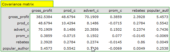
Covariance matrix – similarly to the correlation matrix it contains information about the linear relation among particular variables. That value is not standardized.
Partial correlation coefficient – falls within the range $<-1; 1>$ and is the measure of correlation between the specific independent variable $X_i$ (taking into account its correlation with the remaining variables in the model) and the dependent variable $Y$ (taking into account its correlation with the remaining variables in the model).

The square of that coefficient is the partial determination coefficient – it falls within the range $<0; 1>$ and defines the relation of only the variance of the given independent variable $X_i$ with that variance of the dependent variable $Y$ which was not explained by other variables in the model.

The closer the value of those coefficients to 0, the more useless the information carried by the studied variable, which means the variable is redundant.

Semipartial correlation coefficient – falls within the range $<-1; 1>$ and is the measure of correlation between the specific independent variable $X_i$ (taking into account its correlation with the remaining variables in the model) and the dependent variable $Y$ (NOT taking into account its correlation with the remaining variables in the model).

The square of that coefficient is the semipartial determination coefficient – it falls within the range $<0; 1>$ and defines the relation of only the variance of the given independent variable $X_i$ with the complete variance of the dependent variable $Y$ .

The closer the value of those coefficients to 0, the more useless the information carried by the studied variable, which means the variable is redundants.

R-squared ( $R^2 \in <0; 1>$ ) – it represents the percentage of variance of the given independent variable $X_i$ , explained by the remaining independent variables. The closer to value 1 the stronger the linear relation of the studied variable with the remaining independent variables, which can mean that the variable is a redundant one.
Variance inflation factor ( $VIF \in <1; \infty )$ ) – determines how much the variance of the estimated regression coefficient is increased due to collinearity. The closer the value is to 1, the lower the collinearity and the smaller its effect on the coefficient variance. It is assumed that strong collinearity occurs when the coefficient VIF>5 \cite{sheather}. f the variance inflation factor is 5 ( $\sqrt{5}$ = 2.2), this means that the standard error for the coefficient of this variable is 2.2 times larger than if this variable had zero correlation with other variables $X_i$ .
Tolerance = $1-R^2 \in<0; 1>$ – it represents the percentage of variance of the given independent variable $X_i$ , NOT explained by the remaining independent variables. The closer the value of tolerance is to 0 the stronger the linear relation of the studied variable with the remaining independent variables, which can mean that the variable is a redundant one.
A comparison of a full model with a model in which a given variable is removed

The comparison of the two model is made with by means of:

F test, in a situation in which one variable or more are removed from the model (see: the comparison of models),
t-test, when only one variable is removed from the model. It is the same test that is used for studying the significance of particular variables in the model.

In the case of removing only one variable the results of both tests are identical.

If the difference between the compared models is statistically significant (the value $p \le \alpha$ ), the full model is significantly better than the reduced model. It means that the studied variable is not redundant, it has a significant effect on the given model and should not be removed from it.

Scatter plots

The charts allow a subjective evaluation of linearity of the relation among the variables and an identification of outliers. Additionally, scatter plots can be useful in an analysis of model residuals.

2022/02/09 12:56

Analysis of model residuals

To obtain a correct regression model we should check the basic assumptions concerning model residuals.

Outliers

The study of the model residual can be a quick source of knowledge about outlier values. Such observations can disturb the equation of the regression to a large extent because they have a great effect on the values of the coefficients in the equation. If the given residual $e_i$ deviates by more than 3 standard deviations from the mean value, such an observation can be classified as an outlier. A removal of an outlier can greatly enhance the model.

Cook's distance - describes the magnitude of change in regression coefficients produced by omitting a case. In the program, Cook's distances for cases that exceed the 50th percentile of the F-Snedecor distribution statistic are highlighted in bold $F(0.5, k+1, n-k-1)$ .

Mahalanobis distance - is dedicated to detecting outliers - high values indicate that a case is significantly distant from the center of the independent variables. If a case with the highest Mahalanobis value is found among the cases more than 3 deviations away, it will be marked in bold as the outlier.

Normalność rozkładu reszt modelu

We check this assumption visually using a Q-Q plot of the nromal distribution. The large difference between the distribution of the residuals and the normal distribution may disturb the assessment of the significance of the coefficients of the individual variables in the model.

Homoscedasticity (homogeneity of variance)

To check if there are areas in which the variance of model residuals is increased or decreased we use the charts of:

the residual with respect to predicted values
the square of the residual with respect to predicted values
the residual with respect to observed values
the square of the residual with respect to observed values

Autocorrelation of model residuals

For the constructed model to be deemed correct the values of residuals should not be correlated with one another (for all pairs $e_i, e_j$ ). The assumption can be checked by by computing the Durbin-Watson statistic.

$\begin{displaymath} d=\frac{\sum_{t=2}^n\left(e_t-e_{t-1}\right)^2}{\sum_{t=1}^ne_t^2}, \end{displaymath}$

To test for positive autocorrelation on the significance level $\alpha$ we check the position of the statistics $d$ with respect to the upper ( $d_{U,\alpha}$ ) and lower ( $d_{L,\alpha}$ ) critical value:

If $d <d_{L,\alpha}$ – the errors are positively correlated;
If $d> d_{U,\alpha}$ – the errors are not positively correlated;
If $d_{L,\alpha}<d <d_{U,\alpha}$ – the test result is ambiguous.

To test for negative autocorrelation on the significance level $\alpha$ we check the position of the value $4-d$ with respect to the upper ( $d_{U,\alpha}$ ) and lower ( $d_{L,\alpha}$ ) critical value:

If $4-d <d_{L,\alpha}$ – the errors are negatively correlated;
If $4-d> d_{U,\alpha}$ – the errors are not negatively correlated;
If $d_{L,\alpha}<4-d <d_{U,\alpha}$ – the test result is ambiguous.

The critical values of the Durbin-Watson test for the significance level $\alpha=0.05$ are on the website (pqstat) – the source of the: Savin and White tables (1977)⁶⁾

EXAMPLE cont. (publisher.pqs file)

2022/02/09 12:56

Example for multiple regression

EXAMPLE (publisher.pqs file)

A certain book publisher wanted to learn how was gross profit from sales influenced by such variables as: production cost, advertising costs, direct promotion cost, the sum of discounts made, and the author's popularity. For that purpose he analyzed 40 titles published during the previous year (teaching set). A part of the data is presented in the image below:

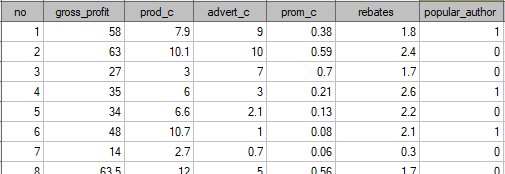
The first five variables are expressed in thousands fo dollars - so they are variables gathered on an interval scale. The last variable: the author's popularity – is a dychotomic variable, where 1 stands for a known author, and 0 stands for an unknown author.

On the basis of the knowledge gained from the analysis the publisher wants to predict the gross profit from the next published book written by a known author. The expenses the publisher will bear are: production cost $\approx 11$ , advertising costs $\approx 13$ , direct promotion costs $\approx 0.5$ , the sum of discounts made $\approx 0.5$ .

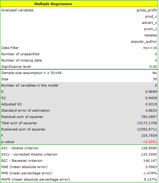
We construct the model of multiple linear regression, for teaching dataset, selecting: gross profit – as the dependent variable $Y$ , production cost, advertising costs, direct promotion costs, the sum of discounts made, the author's popularity – as the independent variables $X_1, X_2, X_3, X_4, X_5$ . As a result, the coefficients of the regression equation will be estimated, together with measures which will allow the evaluation of the quality of the model.

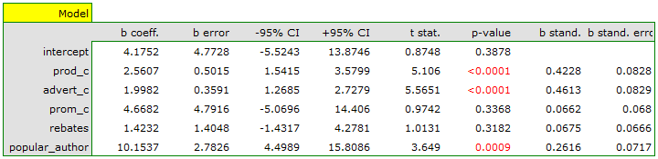
On the basis of the estimated value of the coefficient $b$ , the relationship between gross profit and all independent variables can be described by means of the equation: $\begin{displaymath} profit_{gross}=4.18+2.56(c_{prod})+2(c_{adv})+4.67(c_{prom})+1.42(discounts)+10.15(popul_{author})+[8.09] \end{displaymath}$ The obtained coefficients are interpreted in the following manner:

If the production cost increases by 1 thousand dollars, then gross profit will increase by about 2.56 thousand dollars, assuming that the remaining variables do not change;
If the production cost increases by 1 thousand dollars, then gross profit will increase by about 2 thousand dollars, assuming that the remaining variables do not change;
If the production cost increases by 1 thousand dollars, then gross profit will increase by about 4.67 thousand dollars, assuming that the remaining variables do not change;
If the sum of the discounts made increases by 1 thousand dollars, then gross profit will increase by about 1.42 thousand dollars, assuming that the remaining variables do not change;
If the book has been written by a known author (marked as 1), then in the model the author's popularity is assumed to be the value 1 and we get the equation:

$\begin{displaymath} profit_{gross}=14.33+2.56(c_{prod})+2(c_{adv})+4.67(c_{prom})+1.42(discounts) \end{displaymath}$

If the book has been written by an unknown author (marked as 0), then in the model the author's popularity is assumed to be the value 0 and we get the equation: $\begin{displaymath} profit_{gross}=4.18+2.56(c_{prod})+2(c_{adv})+4.67(c_{prom})+1.42(discounts) \end{displaymath}$

The result of t-test for each variable shows that only the production cost, advertising costs, and author's popularity have a significant influence on the profit gained. At the same time, that standardized coefficients $b$ are the greatest for those variables.

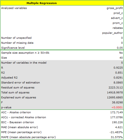
Additionally, the model is very well-fitting, which is confirmed by: the small standard error of estimation $SE_e=8.087$ , the high value of the multiple determination coefficient $R^2=0.85$ , the corrected multiple determination coefficient $R_{adj}^2= 0.83$ , and the result of the F-test of variance analysis: p<0.0001.

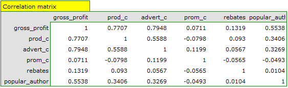
On the basis of the interpretation of the results obtained so far we can assume that a part of the variables does not have a significant effect on the profit and can be redundant. For the model to be well formulated the interval independent variables ought to be strongly correlated with the dependent variable and be relatively weakly correlated with one another. That can be checked by computing the correlation matrix and the covariance matrix:

The most coherent information which allows finding those variables in the model which are redundant is given by the parial and semipartial correlation analysis as well as redundancy analysis:

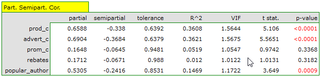
The values of coefficients of partial and semipartial correlation indicate that the smallest contribution into the constructed model is that of direct promotion costs and the sum of discounts made. However, those variables are the least correlated with model residuals, which is indicated by the low value $R^2$ and the high tolerance value. All in all, from the statistical point of view, models without those variables would not be worse than the current model (see the result of t-test for model comparison). The decision about whether or not to leave that model or to construct a new one without the direct promotion costs and the sum of discounts made, belongs to the researcher. We will leave the current model.

Finally, we will analyze the residuals. A part of that analysis is presented below:

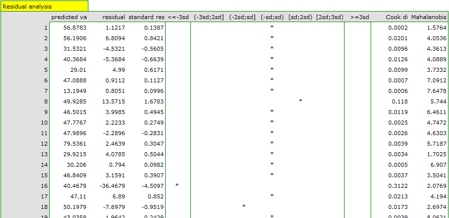
It is noticeable that one of the model residuals is an outlier – it deviates by more than 3 standard deviations from the mean value. It is observation number 16. The observation can be easily found by drawing a chart of residuals with respect to observed or expected values of the variable $Y$ .

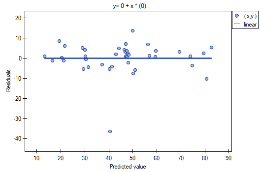
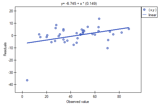
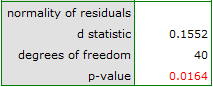
That outlier undermines the assumption concerning homoscedasticity. The assumption of homoscedasticity would be confirmed (that is, residuals variance presented on the axis $Y$ would be similar when we move along the axis $X$ ), if we rejected that point. Additionally, the distribution of residuals deviates slightly from normal distribution (the value $p$ of Liliefors test is p=0.0164):

When we take a closer look of the outlier (position 16 in the data for the task) we see that the book is the only one for which the costs are higher than gross profit (gross profit=4 thousand dollars, the sum of costs = (8+6+0.33+1.6) = 15.93 thousand dollars).

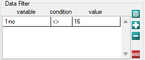
The obtained model can be corrected by removing the outlier. For that purpose, another analysis has to be conducted, with a filter switched on which will exclude the outlier.

As a result, we receive a model which is very similar to the previous one but is encumbered with a smaller error and is more adequate:

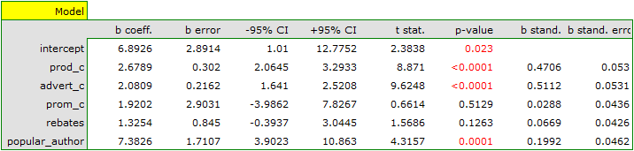
$\begin{displaymath} profit_{gross}=6.89+2.68(c_{prod})+2.08(c_{adv})+1.92(c_{prom})+1.33(discounts)+7.38(popul_{author})+[4.86] \end{displaymath}$

The final version of the model will be used for prediction. On the basis of the predicted costs amounting to: production cost $\approx 11$ thousand dollars,\\advertising costs $\approx 13$ thousand dollars,\\direct promotion costs $\approx 0.5$ thousand dollars,\\the sum of discounts made $\approx 0.5$ thousand dollars,\\and the fact that the author is known (the author's popularity $\approx 1$ ) we calculate the predicted gross profit together with the confidence interval:

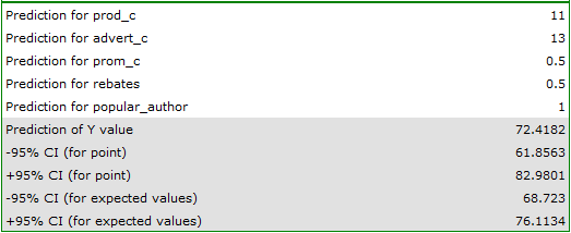
The predicted profit is 72 thousand dollars.

Finally, it should still be noted that this is only a preliminary model. In a proper study more data would have to be collected. The number of variables in the model is too small in relation to the number of books evaluated, i.e. n<50+8k.

2022/02/09 12:56

Model-based prediction and test set validation

Validation

Validation of a model is a check of its quality. It is first performed on the data on which the model was built (the so-called training data set), that is, it is returned in a report describing the resulting model. In order to be able to judge with greater certainty how suitable the model is for forecasting new data, an important part of the validation is to become a model to data that were not used in the model estimation. If the summary based on the treining data is satisfactory, i.e., the determined errors $R^2$ coefficients and information criteria are at a satisfactory level, and the summary based on the new data (the so-called test data set) is equally favorable, then with high probability it can be concluded that such a model is suitable for prediction. The testing data should come from the same population from which the training data were selected. It is often the case that before building a model we collect data, and then randomly divide it into a training set, i.e. the data that will be used to build the model, and a test set, i.e. the data that will be used for additional validation of the model.

The settings window with the validation can be opened in Advanced statistics→Multivariate models→Multiple regression - prediction/validation.

To perform validation, it is necessary to indicate the model on the basis of which we want to perform the validation. Validation can be done on the basis of:

multivariate regression model built in PQStat - simply select a model from the models assigned to the sheet, and the number of variables and model coefficients will be set automatically; the test set should be in the same sheet as the training set;
model not built in PQStat but obtained from another source (e.g., described in a scientific paper we have read) - in the analysis window, enter the number of variables and enter the coefficients for each of them.

In the analysis window, indicate those new variables that should be used for validation.

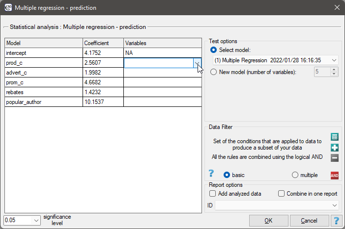
Prediction

Most often, the final step in regression analysis is to use the built and previously validated model for prediction.

Prediction for a single object can be performed along with the construction of the model, that is, in the analysis window Advanced statistics→Multivariate models→Multiple regression ,
Prediction for a larger group of new data is done through the menu Advanced statistics→Multivariate models→Multiple regression - prediction/validation.

To make a prediction, it is necessary to indicate the model on the basis of which we want to make the prediction. Prediction can be made on the basis of:

multivariate regression model built in PQStat -simply select a model from the models assigned to the sheet, and the number of variables and model coefficients will be set automatically; the test set should be in the same sheet as the training set;
model not built in PQStat but obtained from another source (e.g., described in a scientific paper we read) - in the analysis window, the number of variables and the coefficients on each of them should be entered.

In the analysis window, indicate those new variables that should be used for prediction. The estimated value is calculated with some error. Therefore, in addition, for the value predicted by the model, limits are set due to the error:

confidence intervals are set for the expected value,
For a single point, prediction intervals are determined.

Example continued (publisher.pqs file)

To predict gross profit from book sales, the publisher built a regression model based on a training set stripped of item 16 (that is, 39 books). The model included: production costs, advertising costs and author popularity (1=popular author, 0=not). We will build the model once again based on the learning set and then, to make sure the model will work properly, we will validate it on a test data set. If the model passes this test, we will apply it to predictions for book items. To use the right collections we set a data filter each time.

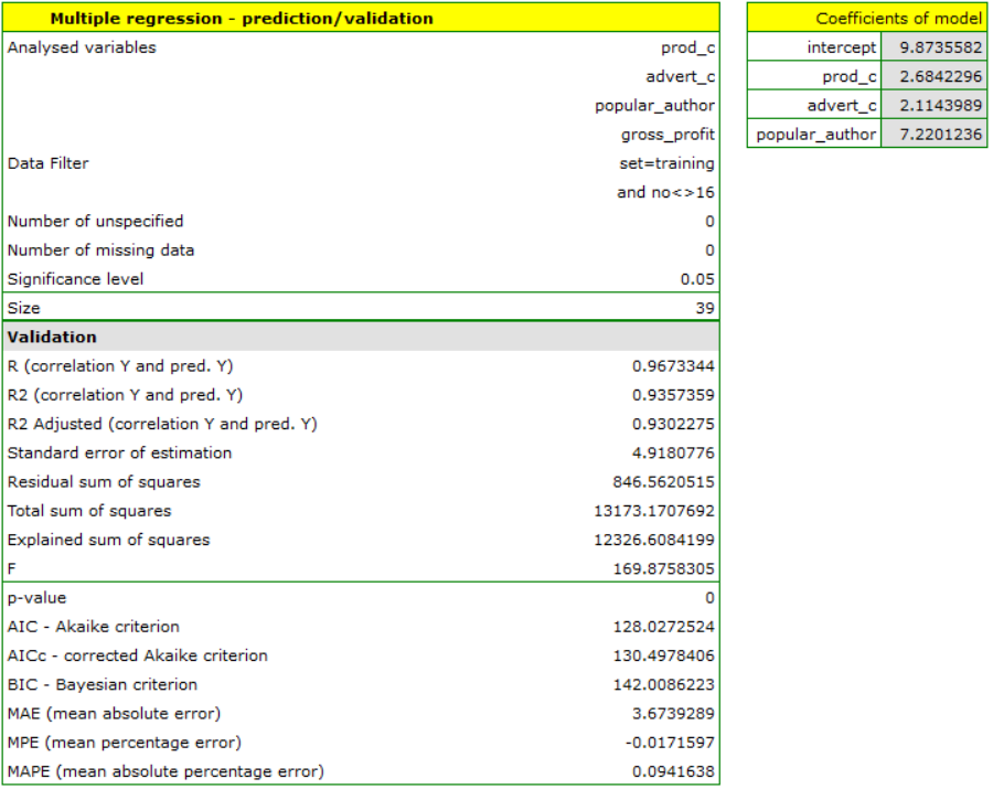
For the training set, the values describing the quality of the model's fit are very high: adjusted $R^2$ = 0.93 and the average forecast error (MAE) is 3.7 thousand dollars.

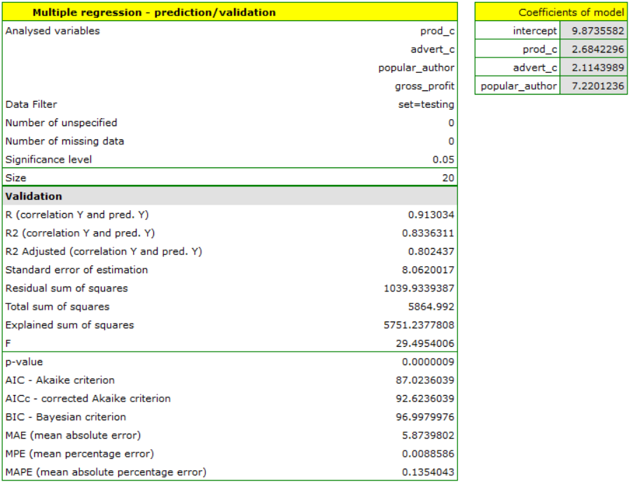
For the test set, the values describing the quality of the model fit are slightly lower than for the learning set: Adjusted $R^2$ = 0.80 and the mean error of prediction (MAE) is 5.9 thousand dollars. Since the validation result on the test set is almost as good as on the training set, we will use the model for prediction. To do this, we will use the data of three new book items added to the end of the set. We'll select Prediction, set filter on the new dataset and use our model to predict the gross profit for these books.

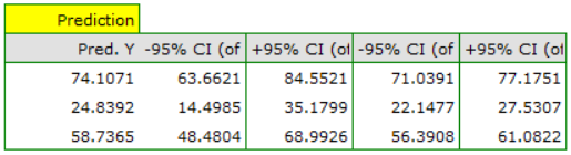
It turns out that the highest gross profit (between 64 and 85 thousands of dollars) is projected for the first, most advertised and most expensive book published by a popular author.

2022/02/09 12:56

Comparison of multiple linear regression models

The window with settings for model comparison is accessed via the menu Advenced statistics→Multidimensional models→Multiple regression – model comparison

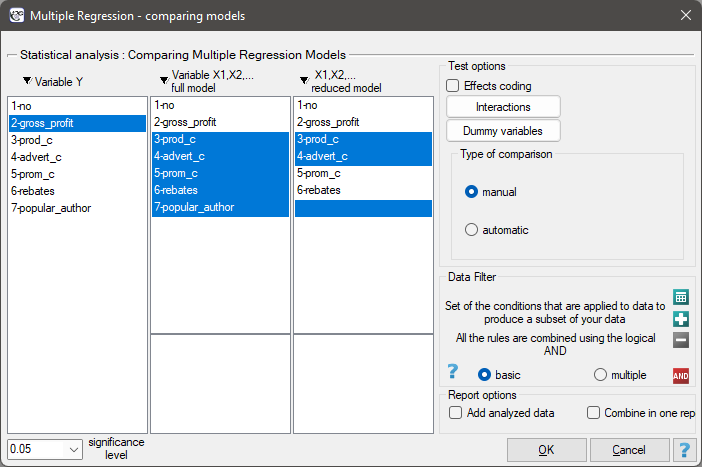
The multiple linear regression offers the possibility of simultaneous analysis of many independent variables. There appears, then, the problem of choosing the optimum model. Too large a model involves a plethora of information in which the important ones may get lost. Too small a model involves the risk of omitting those features which could describe the studied phenomenon in a reliable manner. Because it is not the number of variables in the model but their quality that determines the quality of the model. To make a proper selection of independent variables it is necessary to have knowledge and experience connected with the studied phenomenon. One has to remember to put into the model variables strongly correlated with the dependent variable and weakly correlated with one another.

There is no single, simple statistical rule which would decide about the number of variables necessary in the model. The measures of model adequacy most frequently used in a comparison are: $R_{adj}^2$ – the corrected value of multiple determination coefficient (the higher the value the more adequate the model), $SE_e$ – the standard error of estimation (the lower the value the more adequate the model) or or information criteria AIC, AICc, BIC (the lower the value, the better the model). For that purpose, the F-test based on the multiple determination coefficient $R^2$ can also be used. The test is used to verify the hypothesis that the adequacy of both compared models is equally good.

Hypotheses:

$\begin{array}{cc} \mathcal{H}_0: & R_{FM}^2=R_{RM}^2,\\ \mathcal{H}_1: & R_{FM}^2\ne R_{RM}^2, \end{array}$

where:

$R_{FM}^2, R_{RM}^2$ – multiple determination coefficients in compared models (full and reduced).

The test statistics has the form presented below:

$\begin{displaymath} F=\frac{R_{FM}^2-R_{RM}^2}{k_{FM}-k_{RM}}\cdot\frac{n-k_{FM}-1}{1-R_{FM}^2}, \end{displaymath}$

The statistics is subject to F-Snedecor distribution with $df_1=k_{FM}-k_{RM}$ and $df_2=n-k_{FM}-1$ degrees of freedom.

The p-value, designated on the basis of the test statistic, is compared with the significance level $\alpha$ :

$\begin{array}{ccl} $ if $ p \le \alpha & \Longrightarrow & $ reject $ \mathcal{H}_0 $ and accept $ \mathcal{H}_1, \\ $ if $ p > \alpha & \Longrightarrow & $ there is no reason to reject $ \mathcal{H}_0. \\ \end{array}$

If the compared models do not differ significantly, we should select the one with a smaller number of variables. Because a lack of a difference means that the variables present in the full model but absent from the reduced model do not carry significant information. However, if the difference in the quality of model adequacy is statistically significant, it means that one of them (the one with the greater number of variables, with a greater $R^2$ or lesser value of the information criterion) is significantly better than the other one.

In the program PQStat the comparison of models can be done manually or automatically.

Manual model comparison – construction of 2 models:
- a full model – a model with a greater number of variables,
- a reduced model – a model with a smaller number of variables – such a model is created from the full model by removing those variables which are superfluous from the perspective of studying a given phenomenon.

The choice of independent variables in the compared models and, subsequently, the choice of a better model on the basis of the results of the comparison, is made by the researcher.

Automatic model comparison is done in several steps:

[step 1] Constructing the model with the use of all variables.
[step 2] Removing one variable from the model. The removed variable is the one which, from the statistical point of view, contributes the least information to the current model.
[step 3] A comparison of the full and the reduced model.
[step 4] Removing another variable from the model. The removed variable is the one which, from the statistical point of view, contributes the least information to the current model.
[step 5] A comparison of the previous and the newly reduced model.
[…]

In that way numerous, ever smaller models are created. The last model only contains 1 independent variable.

As a result, each model is described with the help of adequacy measures ( $R_{adj}^2$ , $SE_e$ , AIC, AICc, BIC), and the subsequent (neighboring) models are compared by means of the F-test. The model which is finally marked as statistically best is the model with the greatest $R_{adj}^2$ and the smallest $SE_e$ . However, as none of the statistical methods cannot give a full answer to the question which of the models is the best, it is the researcher who should choose the model on the basis of the results.

EXAMPLE cont. (publisher.pqs file)

To predict the gross profit from book sales a publisher wants to consider such variables as: production cost, advertising costs, direct promotion cost, the sum of discounts made, and the author's popularity. However, not all of those variables need to have a significant effect on profit. Let us try to select such a model of linear regression which will contain the optimum number of variables (from the perspective of statistics). For this analysis, we will use teaching set data.

Manual model comparison.

On the basis of the earlier constructed, full model we can suspect that the variables: direct promotion costs and the sum of discounts made have a small influence on the constructed model (i.e. those variables do not help predict the greatness of the profit). We will check if, from the perspective of statistics, the full model is better than the model from which the two variables have been removed.

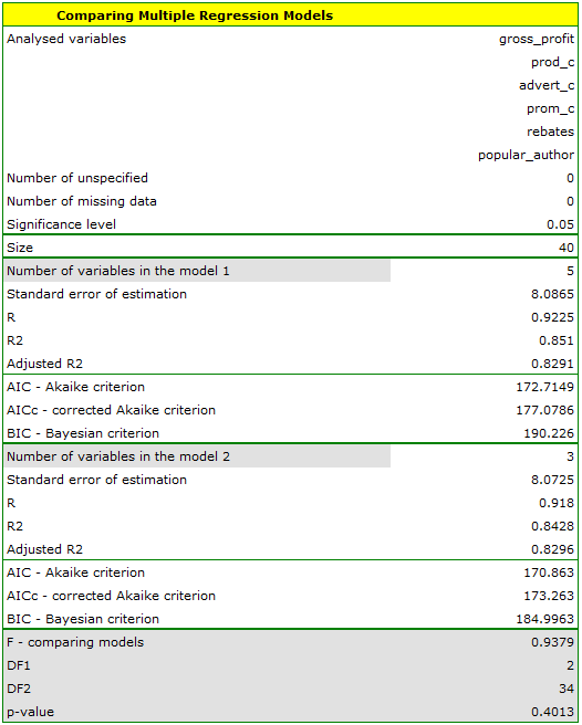
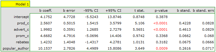
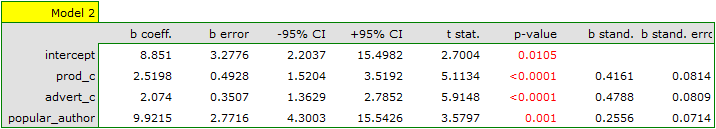
It turns out that there is no basis for thinking that the full model is better than the reduced model (the value $p$ of F-test which is used for comparing models is $p=0.4013$ ). Additionally, the reduced model is slightly more adequate than the full model (for the reduced model $R_{adj}^2=0.8296$ , for the full model $R_{adj}^2=0.8291$ and has smaller, or more favorable, values of the information criteria AIC, AIcc, BIC.

Automatic model comparison.

In the case of automatic model comparison we receive very similar results. The best model is the one with the greatest coefficient $R^2_{adj}$ , the smallest information criteria and the smalles standard estimation error $SE_e$ . The best model we suggest is the model containing only 3 independent variables: the production cost, advertising costs, and the author's popularity. On the basis of the analyses above, from the perspective of statistics, the optimum model is the model with the 3 most important independent variables: the production cost, advertising costs, and the author's popularity. However, the final decision which model to choose should be made by a person with specialist knowledge about the studied topic – in this case, the publisher. It ought to be remembered that the selected model should be constructed anew and its assumptions verified in the window Multiple regression.

2022/02/09 12:56

Logistic regression

The window with settings for Logistic Regression is accessed via the menu Advanced statistics→Multidimensional Models→Logistic Regression

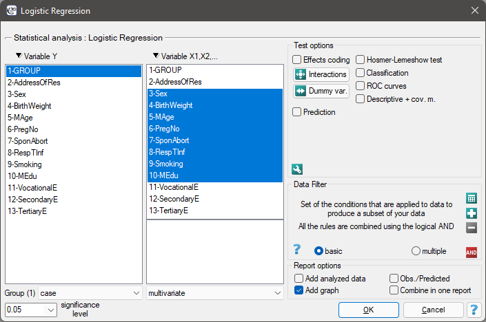
The constructed model of logistic regression (similarly to the case of multiple linear regression) allows the study of the effect of many independent variables ( $X_1, X_2,..., X_k$ ) on one dependent variable( $Y$ ). This time, however, the dependent variable only assumes two values, e.g. ill/healthy, insolvent/solvent etc.

The two values are coded as (1)/(0), where:

(1) the distinguished value - possessing the feature

(0) not possessing the feature.

The function on which the model of logistic regression is based does not calculate the 2-level variable $Y$ but the probability of that variable assuming the distinguished value:

$\begin{displaymath} P(Y=1|X_1,X_2,...,X_k)=\frac{e^Z}{1+e^Z} \end{displaymath}$

where:

$P(Y=1|X_1,X_2,...,X_k)$ - the probability of assuming the distinguished value (1) on condition that specific values of independent variables are achieved, the so-called probability predicted for 1.

$Z$ is most often expressed in the form of a linear relationship:

$Z=\beta_0+\sum_{i=1}^k\beta_iX_i$ ,

$X_1,X_2,\ldots X_k$ - independent variables, explanatory,

$\beta_0,\beta_1,\beta_2,\ldots \beta_k$ - parameters.

Dummy variables and interactions in the model

A discussion of the coding of dummy variables and interactions is presented in chapter Preparation of the variables for the analysis in multidimensional models.

Note Function Z can also be described with the use of a higher order relationship, e.g. a square relationship - in such a case we introduce into the model a variable containing the square of the independent variable $X_i^2$ .

The logit is the transformation of that model into the form:

$\begin{displaymath} \ln\left(\frac{P}{1-P}\right)=Z. \end{displaymath}$

The matrices involved in the equation, for a sample of size $n$ , are recorded in the following manner:

$Y=\left( \begin{array}{ccc} y_1\\ y_2\\ \vdots\\ y_n \end{array} \right),$

$X=\left( \begin{array}{ccccc} 1 & x_{11} & x_{21} & \ldots & x_{k1}\\ 1 & x_{12} & x_{22} & \ldots & x_{k2}\\ \vdots & \vdots & \vdots & \ddots & \vdots\\ 1 & x_{1n} & x_{2n} & \ldots & x_{kn} \end{array} \right),$

$\beta=\left( \begin{array}{ccc} \beta_0\\ \beta_1\\ \beta_2\\ \vdots\\ \beta_k \end{array} \right).$

In such a case, the solution of the equation is the vector of the estimates of parameters $\beta_0,\beta_1,\ldots,\beta_k$ called regression coefficients:

$b=\left( \begin{array}{ccc} b_0\\ b_1\\ b_2\\ \vdots\\ b_k \end{array} \right).$

The coefficients are estimated with the use of the maximum likelihood method, that is through the search for the maximum value of likelihood function $L$ (in the program the Newton-Raphson iterative algorithm was used). On the basis of those values we can infer the magnitude of the effect of the independent variable (for which the coefficient was estimated) on the dependent variable.

There is a certain error of estimation for each coefficient. The magnitude of that error is estimated from the following formula:

$\begin{displaymath} SE_b=\sqrt{diag(H^{-1})_b}, \end{displaymath}$

where:

$diag(H^{-1})$ is the main diagonal of the covariance matrix.

Note When building the model you need remember that the number of observations should be ten times greater than or equal to the number of the estimated parameters of the model ( $n\ge 10(k+1)$ ). However, a more restrictive criterion proposed by P. Peduzzi et al. in 1996⁷⁾ is increasingly used, stating that the number of observations should be ten times or equal to the ratio of the number of independent variables ( $v$ ) and the smaller of the proportion of counts ( $p$ )described from the dependent variable (i.e., proportions of sick or healthy), i.e. ( $n\ge 10v/p$ ).

Note When building the model you need remember that the independent variables should not be collinear. In a case of collinearity estimation can be uncertain and the obtained error values very high. The collinear variables should be removed from the model or one independent variable should be built of them, e.g. instead of the collinear variables of mother age and father age one can build the parents age variable.

Note The criterion of convergence of the function of the Newton-Raphson iterative algorithm can be controlled with the help of two parameters: the limit of convergence iteration (it gives the maximum number of iterations in which the algorithm should reach convergence) and the convergence criterion (it gives the value below which the received improvement of estimation shall be considered to be insignificant and the algorithm will stop).

The Odds Ratio

Individual Odds Ratio

On the basis of many coefficients, for each independent variable in the model an easily interpreted measure is estimated, i.e. the individual Odds Ratio: $\begin{displaymath} OR_i=e^{\beta_i}. \end{displaymath}$

The received Odds Ratio expresses the change of the odds for the occurrence of the distinguished value (1) when the independent variable grows by 1 unit. The result is corrected with the remaining independent variables in the model so that it is assumed that they remain at a stable level while the studied variable is growing by 1 unit.

The OR value is interpreted as follows:

$OR >1$ means the stimulating influence of the studied independent variable on obtaining the distinguished value (1), i.e. it gives information about how much greater are the odds of the occurrence of the distinguished value (1) when the independent variable grows by 1 unit.
$OR <1$ means the destimulating influence of the studied independent variable on obtaining the distinguished value (1), i.e. it gives information about how much lower are the odds of the occurrence of the distinguished value (1) when the independent variable grows by 1 unit.
$OR\approx1$ means that the studied independent variable has no influence on obtaining the distinguished value (1).

Odds Ratio - the general formula

The PQStat program calculates the individual Odds Ratio. Its modification on the basis of a general formula makes it possible to change the interpretation of the obtained result.

The Odds Ratio for the occurrence of the distinguished state in a general case is calculated as the ratio of two odds. Therefore for the independent variable $X_1$ for $Z$ expressed with a linear relationship we calculate:

the odds for the first category: $\begin{displaymath} Odds(1)=\frac{P(1)}{1-P(1)}=e^Z(1)=e^{\beta_0+\beta_1X_1(1)+\beta_2X_2+...+\beta_kX_k}, \end{displaymath}$

the odds for the second category:

$\begin{displaymath} Odds(2)=\frac{P(2)}{1-P(2)}=e^Z(2)=e^{\beta_0+\beta_1X_1(2)+\beta_2X_2+...+\beta_kX_k}. \end{displaymath}$

The Odds Ratio for variable $X_1$ is then expressed with the formula:

$\begin{displaymath} \begin{array}{lll} OR_1(2)/(1) &=&\frac{Odds(2)}{Odds(1)}=\frac{e^{\beta_0+\beta_1X_1(2)+\beta_2X_2+...+\beta_kX_k}}{e^{\beta_0+\beta_1X_1(1)+\beta_2X_2+...+\beta_kX_k}}\\ &=& e^{\beta_0+\beta_1X_1(2)+\beta_2X_2+...+\beta_kX_k-[\beta_0+\beta_1X_1(1)+\beta_2X_2+...+\beta_kX_k]}\\ &=& e^{\beta_1X_1(2)-\beta_1X_1(1)}=e^{\beta_1[X_1(2)-X_1(1)]}=\\ &=& \left(e^{\beta_1}\right)^{[X_1(2)-X_1(1)]}. \end{array} \end{displaymath}$

Example

If the independent variable is age expressed in years, then the difference between neighboring age categories such as 25 and 26 years is 1 year $\left(X_1(2)-X_1(1)=26-25=1\right)$ . In such a case we will obtain the individual Odds Ratio:

$\begin{displaymath}OR=\left(e^{\beta_1}\right)^1,\end{displaymath}$

which expresses the degree of change of the odds for the occurrence of the distinguished value if the age is changed by 1 year.

The odds ratio calculated for non-neighboring variable categories, such as 25 and 30 years, will be a five-year Odds Ratio, because the difference $X_1(2)-X_1(1)=30-25=5$ . In such a case we will obtain the five-year Odds Ratio:

$\begin{displaymath}OR=\left(e^{\beta_1}\right)^5,\end{displaymath}$

which expresses the degree of change of the odds for the occurrence of the distinguished value if the age is changed by 5 years.

Note

If the analysis is made for a non-linear model or if interaction is taken into account, then, on the basis of a general formula, we can calculate an appropriate Odds Ratio by changing the formula which expresses $Z$ .

EXAMPLE cont. (task.pqs file)

EXAMPLE cont. (anomaly.pqs file)

2022/02/09 12:56

Model verification

Statistical significance of particular variables in the model (significance of the Odds Ratio)

On the basis of the coefficient and its error of estimation we can infer if the independent variable for which the coefficient was estimated has a significant effect on the dependent variable. For that purpose we use Wald test.

Hypotheses:

$\begin{array}{cc} \mathcal{H}_0: & \beta_i=0,\\ \mathcal{H}_1: & \beta_i\ne 0. \end{array}$

or, equivalently:

$\begin{array}{cc} \mathcal{H}_0: & OR_i=1,\\ \mathcal{H}_1: & OR_i\ne 1. \end{array}$

The Wald test statistics is calculated according to the formula:

$\begin{displaymath} \chi^2=\left(\frac{b_i}{SE_{b_i}}\right)^2 \end{displaymath}$

The statistic asymptotically (for large sizes) has the Chi-square distribution with $1$ degree of freedom.

The p-value, designated on the basis of the test statistic, is compared with the significance level $\alpha$ :

$\begin{array}{ccl} $ if $ p \le \alpha & \Longrightarrow & $ reject $ \mathcal{H}_0 $ and accept $ \mathcal{H}_1, \\ $ if $ p > \alpha & \Longrightarrow & $ there is no reason to reject $ \mathcal{H}_0. \\ \end{array}$

The quality of the constructed model

A good model should fulfill two basic conditions: it should fit well and be possibly simple. The quality of multiple linear regression can be evaluated can be evaluated with a few general measures based on: $L_{FM}$ - the maximum value of likelihood function of a full model (with all variables),

$L_0$ - the maximum value of the likelihood function of a model which only contains one free word,

$n$ - the sample size.

Information criteria are based on the information entropy carried by the model (model insecurity), i.e. they evaluate the lost information when a given model is used to describe the studied phenomenon. We should, then, choose the model with the minimum value of a given information criterion.

$AIC$ , $AICc$ , and $BIC$ is a kind of a compromise between the good fit and complexity. The second element of the sum in formulas for information criteria (the so-called penalty function) measures the simplicity of the model. That depends on the number of variables ( $k$ ) in the model and the sample size ( $n$ ). In both cases the element grows with the increase of the number of variables and the growth is the faster the smaller the number of observations. The information criterion, however, is not an absolute measure, i.e. if all the compared models do not describe reality well, there is no use looking for a warning in the information criterion.

Akaike information criterion

$\begin{displaymath} AIC=-2\ln L_{FM}+2k, \end{displaymath}$

It is an asymptomatic criterion, appropriate for large sample sizes.

Corrected Akaike information criterion

$\begin{displaymath} AICc=AIC+\frac{2k(k+1)}{n-k-1}, \end{displaymath}$

Because the correction of the Akaike information criterion concerns the sample size it is the recommended measure (also for smaller sizes).

Bayesian information criterion or Schwarz criterion

$\begin{displaymath} BIC=-2\ln L_{FM}+k\ln(n), \end{displaymath}$

Just like the corrected Akaike criterion it takes into account the sample size.

Pseudo R $^2$ - the so-called McFadden R $^2$ is a goodness of fit measure of the model (an equivalent of the coefficient of multiple determination $R^2$ defined for multiple linear regression).

The value of that coefficient falls within the range of $<0; 1)$ , where values close to 1 mean excellent goodness of fit of a model, $0$ - a complete lack of fit Coefficient $R^2_{Pseudo}$ is calculated according to the formula:

$\begin{displaymath} R^2_{Pseudo}=1-\frac{\ln L_{FM}}{\ln L_0}. \end{displaymath}$

As coefficient $R^2_{Pseudo}$ never assumes value 1 and is sensitive to the amount of variables in the model, its corrected value is calculated:

$\begin{displaymath} R^2_{Nagelkerke}=\frac{1-e^{-(2/n)(\ln L_{FM}-\ln L_0)}}{1-e^{(2/n)\ln L_0}} \quad \textrm{lub}\quad R^2_{Cox-Snell}=1-e^{\frac{(-2\ln L_0)-(-2\ln L_{FM})}{n}}. \end{displaymath}$

Statistical significance of all variables in the model

The basic tool for the evaluation of the significance of all variables in the model is the Likelihood Ratio test. The test verifies the hypothesis:

$\begin{array}{cc} \mathcal{H}_0: & \textrm{all }\beta_i=0,\\ \mathcal{H}_1: & \textrm{there is }\beta_i\neq0. \end{array}$

The test statistic has the form presented below:

$\begin{displaymath} \chi^2=-2\ln(L_0/L_{FM})=-2\ln(L_0)-(-2\ln(L_{FM})). \end{displaymath}$

The statistic asymptotically (for large sizes) has the Chi-square distribution with $k$ degrees of freedom.

The p-value, designated on the basis of the test statistic, is compared with the significance level $\alpha$ :

$\begin{array}{ccl} $ if $ p \le \alpha & \Longrightarrow & $ reject $ \mathcal{H}_0 $ and accept $ \mathcal{H}_1, \\ $ if $ p > \alpha & \Longrightarrow & $ there is no reason to reject $ \mathcal{H}_0. \\ \end{array}$

Hosmer-Lemeshow test - The test compares, for various subgroups of data, the observed rates of occurrence of the distinguished value $O_g$ and the predicted probability $E_g$ . If $O_g$ and $E_g$ are close enough then one can assume that an adequate model has been built.

For the calculation the observations are first divided into $G$ subgroups - usually deciles ( $G=10$ ).

Hypotheses:

$\begin{array}{cl} \mathcal{H}_0: & O_g=E_g $ for all categories,$\\ \mathcal{H}_1: & O_g \neq E_g $ for at least one category.$ \end{array}$

The test statistic has the form presented below:

$\begin{displaymath} H=\sum_{g=1}^G\frac{(O_g-E_g)^2}{E_g(1-\frac{E_g}{N_g})}, \end{displaymath}$

where:

$N_g$ - the number of observations in group $g$ .

The statistic asymptotically (for large sizes) has the Chi-square distribution with $G-2$ degrees of freedom.

The p-value, designated on the basis of the test statistic, is compared with the significance level $\alpha$ :

$\begin{array}{ccl} $ if $ p \le \alpha & \Longrightarrow & $ reject $ \mathcal{H}_0 $ and accept $ \mathcal{H}_1, \\ $ if $ p > \alpha & \Longrightarrow & $ there is no reason to reject $ \mathcal{H}_0. \\ \end{array}$

AUC - the area under the ROC curve - The ROC curve built on th ebasis of the value of the dependent variable, and the predicted probability of dependent variable $P$ , allows to evaluate the ability of the constructed logistic regression model to classify the cases into two groups: (1) and (0). The constructed curve, especially the area under the curve, presents the classification quality of the model. When the ROC curve overlaps with the diagonal $y = x$ , then the decision about classifying a case within a given class (1) or (0), made on the basis of the model, is as good as a random division of the studied cases into the groups. The classification quality of a model is good when the curve is much above the diagonal $y = x$ , that is when the area under the ROC curve is much larger than the area under the $y = x$ line, i.e. it is greater than $0.5$

Hypotheses:

$\begin{array}{cl} \mathcal{H}_0: & AUC=0.5, \\ \mathcal{H}_1: & AUC\neq 0.5. \end{array}$

The test statistic has the form presented below:

$\begin{displaymath} Z=\frac{AUC-0.5}{SE_{0.5}}, \end{displaymath}$

where:

$SE_{0.5}$ - area error.

Statistics $Z$ asymptotically (for large sizes) has the normal distribution.

The p-value, designated on the basis of the test statistic, is compared with the significance level $\alpha$ :

$\begin{array}{ccl} $ if $ p \le \alpha & \Longrightarrow & $ reject $ \mathcal{H}_0 $ and accept $ \mathcal{H}_1, \\ $ if $ p > \alpha & \Longrightarrow & $ there is no reason to reject $ \mathcal{H}_0. \\ \end{array}$

Additionally, for ROC curve the suggested value of the cut-off point of the predicted probability is given, together with the table of sensitivity and specificity for each possible cut-off point.

Note!

More possibilities of calculating a cut-off point are offered by module **ROC curve**. The analysis is made on the basis of observed values and predicted probability obtained in the analysis of Logistic Regression.

Classification

On the basis of the selected cut-off point of predicted probability we can change the classification quality. By default the cut-off point has the value of 0.5. The user can change the value into any value from the range of $(0.1)$ , e.g. the value suggested by the ROC curve.

As a result we shall obtain the classification table and the percentage of properly classified cases, the percentage of properly classified (0) - specificity, and the percentage of properly classified (1) - sensitivity.

2022/02/09 12:56

Graphs in logistic regression

Odds Ratio with confidence interval – is a graph showing the OR along with the 95 percent confidence interval for the score of each variable returned in the constructed model. For categorical variables, the line at level 1 indicates the odds ratio value for the reference category.

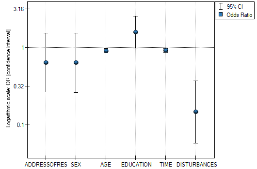
Observed Values / Expected Probability – is a graph showing the results of each person's predicted probability of an event occurring (X-axis) and the true value, which is the occurrence of the event (value 1 on the Y-axis) or the absence of the event (value 0 on the Y-axis). If the model predicts very well, points will accumulate at the bottom near the left side of the graph and at the top near the right side of the graph.

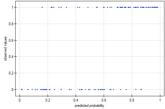
ROC curve – is a graph constructed based on the value of the dependent variable and the predicted probability of an event.

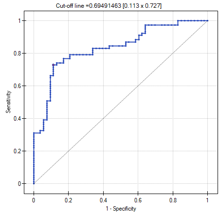
Pearson residuals plot – is a graph that allows you to assess whether there are outliers in the data. The residuals are the differences between the observed value and the probability predicted by the model. Plots of raw residuals from logistic regression are difficult to interpret, so they are unified by determining Pearson residuals. The Pearson residual is the raw residual divided by the square root of the variance function. The sign (positive or negative) indicates whether the observed value is higher or lower than the value fitted to the model, and the magnitude indicates the degree of deviation. Person's residuals less than or greater than 3 suggest that the variance of a given object is too largeu.

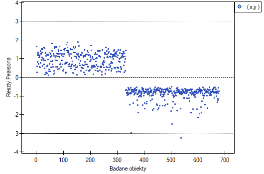
Unit changes in the odds ratio – is a graph showing a series of odds ratios, along with a confidence interval, determined for each possible cut-off point of a variable placed on the X axis. It allows the user to select one good cut-off point and then build from that a new bivariate variable at which a high or low odds ratio is achieved, respectively. The chart is dedicated to the evaluation of continuous variables in univariate analysis, i.e. when only one independent variable is selected.
odds ratio profile is a graph presenting series of odds ratios with confidence interval, determined for a given window size, i.e. comparing frequencies inside the window with frequencies placed outside the window. It enables the user to choose several categories into which he wants to divide the examined variable and adopt the most advantageous reference category. It works best when we are looking for a U-shaped function i.e. high risk at low and at high values of the variable under study and low risk at average values. There is no one window size that is good for every analysis, the window size must be determined individually for each variable. The size of the window indicates the number of unique values of variable X contained in the window. The wider the window, the greater the generalizability of the results and the smoother the odds ratio function. The narrower the window, the more detailed the results, resulting in a more lopsided odds ratio function. A curve is added to the graph showing the smoothed (Lowess method) odds ratio value. Setting the smoothing factor close to 0 results in a curve closely fitting to the odds ratio, whereas setting the smoothing factor closer to 1 results in more generalized odds ratio, i.e. smoother and less fitting to the odds ratio curve. The graph is dedicated to the evaluation of continuous variables in univariate analysis, i.e. when only one independent variable is selected.

EXAMPLE (OR profiles.pqs file)

We examine the risk of disease A and disease B as a function of the patient's BMI. Since BMI is a continuous variable, its inclusion in the model results in a unit odds ratio that determines a linear trend of increasing or decreasing risk. We do not know whether a linear model will be a good model for the analysis of this risk, so before building multivariate logistic regression models, we will build some univariate models presenting this variable in graphs to be able to assess the shape of the relationship under study and, based on this, decide how we should prepare the variable for analysis. For this purpose, we will use plots of unit changes in odds ratio and odds ratio profiles, and for the profiles we will choose a window size of 100 because almost every patient has a different BMI, so about 100 patients will be in each window.

Disease A

Unit changes in the odds ratio show that when the BMI cut-off point is chosen somewhere between 27 and 37, we get a statistically significant and positive odds ratio showing that people with a BMI above this value have a significantly higher risk of disease than people below this value.

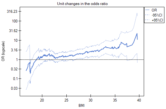
The odds ratio profiles show that the red curve is still close to 1, only the top of the curve is slightly higher, indicating that it may be difficult to divide BMI into more than 2 categories and select a good reference category, i.e., one that yields significant odds ratios.

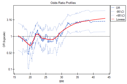
In summary, one can use a split of BMI into two values (e.g., relate those with a BMI above 30 to those with a BMI below that, in which case OR[95%CI]=[1.41, 4.90], p=0.0024) or stay with the unit odds ratio, indicating a constant increase in disease risk with an increase in BMI of one unit (OR[95%CI]=1.07[1.02, 1.13], p=0.0052).

Disease B

Unit changes in the odds ratio show that when the BMI cut-off point is chosen somewhere between 22 and 35, we get a statistically significant and positive odds ratio showing that people with a BMI above this value have a significantly higher risk of disease than those below this value.

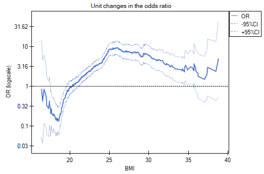
The odds ratio profiles show that it would be much better to divide BMI into 2 or 4 categories. With the reference category being the one that includes a BMI somewhere between 19 and 25, as this is the category that is lowest and is far removed from the results for BMIs to the left and right of this range. We see a distinct U-like shape, meaning that disease risk is high at low BMI and at high BMI.

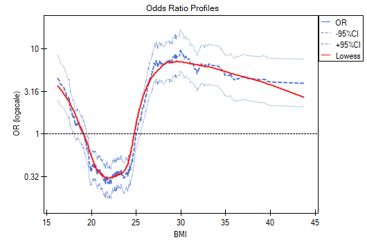
In summary, although the relationship for the unit odds ratio, or linear relationship, is statistically significant, it is not worth building such a model. It is much better to divide BMI into categories. The division that best shows the shape of this relationship is the one using two or three BMI categories, where the reference value will be the average BMI. Using the standard division of BMI and establishing a reference category of BMI in the normal range will result in a more than 15 times higher risk for underweight people (OR[95%CI]=15.14[6.93, 33.10]) more than 10 times for overweight people (OR[95%CI]=10.35[6.74, 15.90]) and more than twelve times for people with obesity (OR[95%CI]=12.22[6.94, 21.49]).

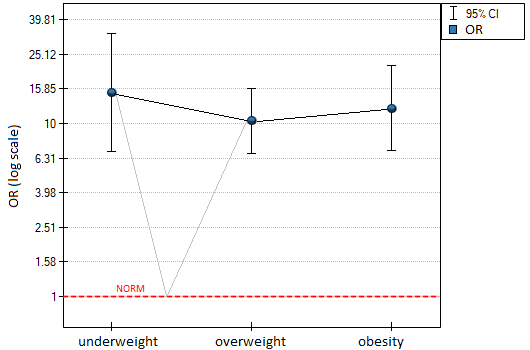
In the odds ratio plot, the BMI norm is indicated at level 1, as the reference category. We have drawn lines connecting the obtained ORs and also the norm, so as to show that the obtained shape of the relationship is the same as that determined previously by the odds ratio profile.

2022/02/09 12:56

Examples for logistic regression

EXAMPLE (anomaly.pqs file)

Studies have been conducted for the purpose of identifying the risk factors for a certain rare congenital anomaly in children. 395 mothers of children with that anomaly and 375 of healthy children have participated in that study. The gathered data are: address of residence, child's sex, child's weight at birth, mother's age, number of pregnancy, previous spontaneous abortions, respiratory tract infections, smoking, mother's education.

We construct a logistic regression model to check which variables may have a significant influence on the occurrence of the anomaly. The dependent variable is the column GROUP, the distinguished values in that variable as $1$ are the cases, that are mothers of children with anomaly. The following $9$ variables are independent variables:

AddressOfRes (2=city/1=village),

Sex (1=male/0=female),

BirthWeight (in kilograms, with an accuracy of 0.5 kg),

MAge (in years),

PregNo (which pregnancy is the child from),

SponAbort (1=yes/0=no),

RespTInf (1=yes/0=no),

Smoking (1=yes/0=no),

MEdu (1=primary or lower/2=vocational/3=secondary/4=tertiary).

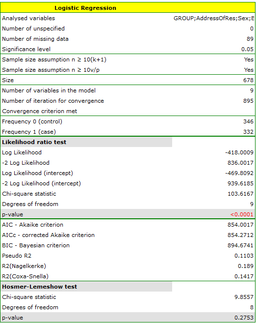
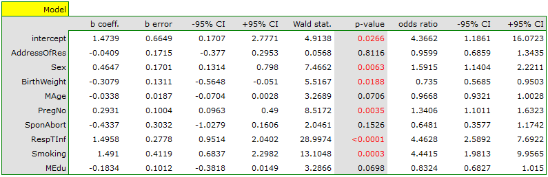
The quality of model goodness of fit is not high ( $R^2_{Pseudo}=0.11$ , $R^2_{Nagelkerke}=0.19$ i $R^2_{Cox-Snell}=0.14$ ). At the same time the model is statistically significant (value $p<0.000001$ of the Likelihood Ratio test), which means that a part of the independent variables in the model is statistically significant. The result of the Hosmer-Lemeshow test points to a lack of significance ( $p=0.2753$ ). However, in the case of the Hosmer-Lemeshow test we ought to remember that a lack of significance is desired as it indicates a similarity of the observed sizes and of predicted probability.

An interpretation of particular variables in the model starts from checking their significance. In this case the variables which are significantly related to the occurrence of the anomaly are:

Sex: $p=0.0063$ ,

BirthWeight: $p=0.0188$ ,

PregNo: $p=0.0035$ ,

RespTInf: $p<0.000001$ ,

Smoking: $p=0.0003$ .

The studied congenital anomaly is a rare anomaly but the odds of its occurrence depend on the variables listed above in the manner described by the odds ratio:

variable Sex: $OR[95%CI]=1.60[1.14;2.22]$ \textendash the odds of the occurrence of the anomaly in a boy is $1.6$ times greater than in a girl;
variable BirthWeight: $OR[95%CI]=0.74[0.57;0.95]$ \textendash the higher the birth weight the smaller the odds of the occurrence of the anomaly in a child;
variable PregNo: $OR[95%CI]=1.34[1.10;1.63]$ \textendash the odds of the occurrence of the anomaly in a child is $1.34$ times greater with each subsequent pregnancy;
variable RespTInf: $OR[95%CI]=4.46[2.59;7.69]$ \textendash the odds of the occurrence of the anomaly in a child if the mother had a respiratory tract infection during the pregnancy is $4.46$ times greater than in a mother who did not have such an infection during the pregnancy;
variable Smoking: $OR[95%CI]=4.44[1.98;9.96]$ \textendash a mother who smokes when pregnant increases the risk of the occurrence of the anomaly in her child $4.44$ times.

In the case of statistically insignificant variables the confidence interval for the Odds Ratio contains 1 which means that the variables neither increase nor decrease the odds of the occurrence of the studied anomaly. Therefore, we cannot interpret the obtained ratio in a manner similar to the case of statistically significant variables.

The influence of particular independent variables on the occurrence of the anomaly can also be described with the help of a chart concerning the odds ratio:

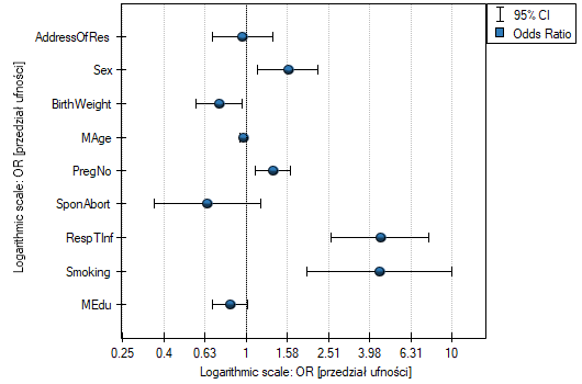
EXAMPLE continued (anomaly.pqs file)

Let us once more construct a logistic regression model, however, this time let us divide the variable mother's education into dummy variables (with dummy coding). With this operation we lose the information about the ordering of the category of education but we gain the possibility of a more in-depth analysis of particular categories. The breakdown into dummy variables is done by selecting Dummy var. in the analysis window.:

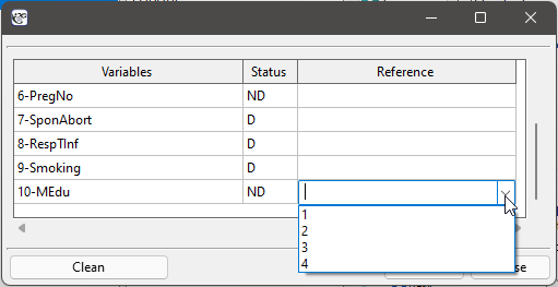
The primary education variable is missing as it will constitute the reference category.

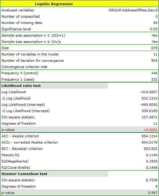
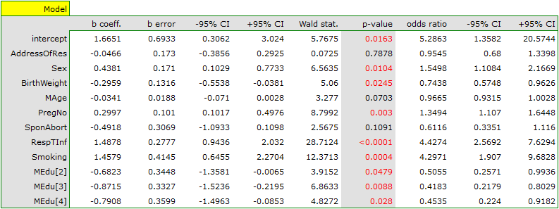
As a result the variables which describe education become statistically significant. The goodness of fit of the model does not change much but the manner of interpretation of the the odds ratio for education does change:

$\begin{tabular}{|l|l|} \hline \textbf{Variable}& $OR[95\%CI]$ \\\hline Primary education& reference category\\ Vocational education& $0.51[0.26;0.99]$\\ Secondary education& $0.42[0.22;0.80]$\\ Tertiary education& $0.45[0.22;0.92]$\\\hline \end{tabular}$

The odds of the occurrence of the studied anomaly in each education category is always compared with the odds of the occurrence of the anomaly in the case of primary education. We can see that for more educated the mother, the odds is lower. For a mother with:

vocational education the odds of the occurrence of the anomaly in a child is 0.51 of the odds for a mother with primary education;
secondary education the odds of the occurrence of the anomaly in a child is 0.42 of the odds for a mother with primary education;
tertiary education the odds of the occurrence of the anomaly in a child is 0.45 of the odds for a mother with primary education;

EXAMPLE (task.pqs file)

An experiment has been made with the purpose of studying the ability to concentrate of a group of adults in an uncomfortable situation. 190 people have taken part in the experiment (130 people are the teaching set, 40 people are the test set). Each person was assigned a certain task the completion of which requried concentration. During the experiment some people were subject to a disturbing agent in the form of temperature increase to 32 degrees Celsius. The participants were also asked about their address of residence, sex, age, and education. The time for the completion of the task was limited to 45 minutes. In the case of participants who completed the task before the deadline, the actual time devoted to the completion of the task was recorded. We will perform all our calculations only for those belonging to the teaching set. }

Variable SOLUTION (yes/no) contains the result of the experiment, i.e. the information about whether the task was solved correctly or not. The remaining variables which could have influenced the result of the experiment are:

ADDRESSOFRES (1=city/0=village),

SEX (1=female/0=male),

AGE (in years),

EDUCATION (1=primary, 2=vocational, 3=secondary, 4=tertiary),

TIME needed for the completion of the task (in minutes),

DISTURBANCES (1=yes/0=no).

On the basis of all those variables a logistic regression model was built in which the distinguished state of the variable SOLUTION was set to „yes”.

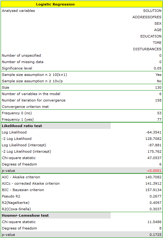
The adequacy quality is described by the coefficients: $R^2_{Pseudo}=0.27$ , $R^2_{Nagelkerke}=0.41$ i $R^2_{Cox-Snell}=0.30$ . The sufficient adequacy is also indicated by the result of the Hosmer-Lemeshow test $(p=0.1725)$ . The whole model is statistically significant, which is indicated by the result of the Likelihood Ratio test $(p<0.000001)$ .

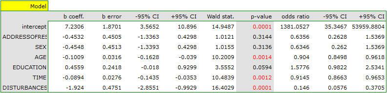
The observed values and predicted probability can be observed on the chart:

In the model the variables which have a significant influence on the result are:

AGE: p=0.0014,

TIME: p=0.0012,

DISTURBANCES: <p=0.0001.

What is more, the younger the person who solves the task the shorter the time needed for the completion of the task, and if there is no disturbing agent, the probability of correct solution is greater:

AGE: $OR[95%CI]=0.90[0.85;0.96]$ ,

TIME: $OR[95%CI]=0.91[0.87;0.97]$ ,

DISTURBANCES: $OR[95%CI]=0.15[0.06;0.37]$ .

The obtained results of the Odds Ratio are presented on the chart below:

Should the model be used for prediction, one should pay attention to the quality of classification. For that purpose we calculate the ROC curves.

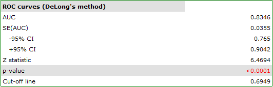
The result seems satisfactory. The area under the curve is $AUC=0.83$ and is statistically greater than $0.5$ $(p<0.0001)$ , so classification is possible on the basis of the constructed model. The suggested cut-off point for the ROC curve is $0.6949$ and is slightly higher than the standard level used in regression, i.e. $0.5$ . The classification determined from this cut-off point yields $79.23%$ of cases classified correctly, of which correctly classified yes values are $72.73%$ (sensitivity), no values are $88.68%$ (specificity). The classification derived from the standard value yields no less, $73.85%$ of cases classified correctly, but it will yield more correctly classified yes values are $83.12%$ , although less correctly classified no values are $60.38\%$ .

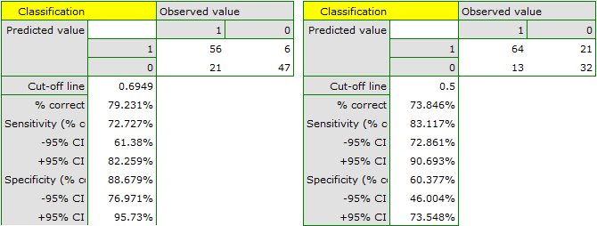
We can finish the analysis of classification at this stage or, if the result is not satisfactory, we can make a more detailed analysis of the ROC curve in module ROC curve.

As we have assumed that classification on the basis of that model is satisfactory we can calculate the predicted value of a dependent variable for any conditions. Let us check what odds of solving the task has a person whose:

ADDRESSOFRES (1=city),

SEX (1=female),

AGE (50 years),

EDUCATION (1=primary),

TIME needed for the completion of the task (20 minutes),

DISTURBANCES (1=yes).

For that purpose, on the basis of the value of coefficient $b$ , we calculate the predicted probability (probability of receiving the answer „yes” on condition of defining the values of dependent variables):

$\begin{displaymath} \begin{array}{l} P(Y=yes|ADDRESSOFRES,SEX,AGE,EDUCATION,TIME,DISTURBANCES)=\\[0.2cm] =\frac{e^{7.23-0.45\textrm{\scriptsize \textit{ADDRESSOFRES}}-0.45\textrm{\scriptsize\textit{SEX}}-0.1\textrm{\scriptsize\textit{AGE}}+0.46\textrm{\scriptsize\textit{EDUCATION}}-0.09\textrm{\scriptsize\textit{TIME}}-1.92\textrm{\scriptsize\textit{DISTURBANCES}}}}{1+e^{7.23-0.45\textrm{\scriptsize\textit{ADDRESSOFRES}}-0.45\textrm{\scriptsize\textit{SEX}}-0.1\textrm{\scriptsize\textit{AGE}}+0.46\textrm{\scriptsize\textit{EDUCATION}}-0.09\textrm{\scriptsize\textit{TIME}}-1.92\textrm{\scriptsize\textit{DISTURBANCES}}}}=\\[0.2cm] =\frac{e^{7.231-0.453\cdot1-0.455\cdot1-0.101\cdot50+0.456\cdot1-0.089\cdot20-1.924\cdot1}}{1+e^{7.231-0.453\cdot1-0.455\cdot1-0.101\cdot50+0.456\cdot1-0.089\cdot20-1.924\cdot1}} \end{array} \end{displaymath}$

As a result of the calculation the program will return the result:

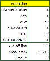
The obtained probability of solving the task is equal to $0.1215$ , so, on the basis of the cut-off $0.60$ , the predicted result is $0$ \textendash which means the task was not solved correctly.

2022/02/09 12:56

Model-based prediction and test set validation

Validation

Validation of a model is a check of its quality. It is first performed on the data on which the model was built (the so-called training data set), that is, it is returned in a report describing the resulting model. To be able to judge with greater certainty how suitable the model is for forecasting new data, an important part of the validation is to apply the model to data that were not used in the model estimation. If the summary based on the training data is satisfactory, i.e. the determined errors, $R^2$ coefficients and information criteria are at a satisfactory level, and the summary based on the new data (the so-called test data set) is equally favorable, then with high probability it can be concluded that such a model is suitable for prediction. The test data should come from the same population from which the training data were selected. It is often the case that before building a model we collect data, and then randomly divide it into a training set, i.e. the data that will be used to build the model, and a test set, i.e. the data that will be used for additional validation of the model.
The settings window with the validation can be opened in Advanced statistics→Multivariate models→Logistic regression - prediction/validation.

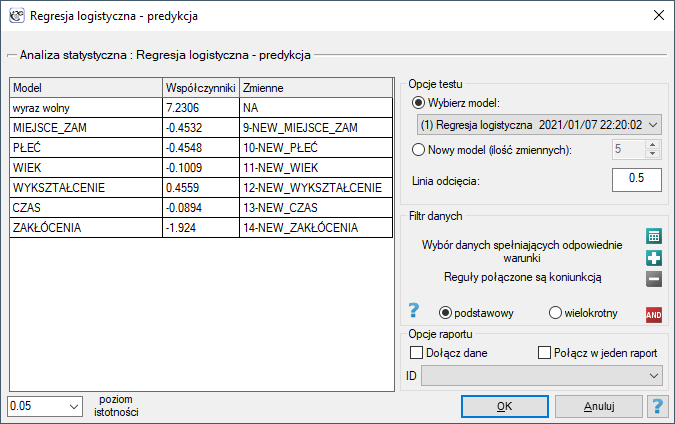
To perform validation, it is necessary to indicate the model on the basis of which we want to perform the validation. Validation can be done on the basis of:

logistic regression model built in PQStat - simply select a model from the models assigned to the sheet, and the number of variables and model coefficients will be set automatically; the test set should be in the same sheet as the training set;
model not built in PQStat but obtained from another source (e.g., described in a scientific paper we have read) - in the analysis window, enter the number of variables and enter the coefficients for each of them.

In the analysis window, indicate those new variables that should be used for validation.

Prediction

Most often, the final step in regression analysis is to use the built and previously validated model for prediction.

Prediction for a single object can be performed along with model building, that is, in the analysis window Advanced statistics→Multivariate models→Logistic regression ,
Predykcja dla większej grupy nowych danych jest wykonywana poprzez menuAdvanced statistics→Multivariate models→Logistic regression - prediction/validation.

To make a prediction, it is necessary to indicate the model on the basis of which we want to make the prediction. Prediction can be made on the basis of:

logistic regression model built in PQStat - simply select a model from the models assigned to the sheet, and the number of variables and model coefficients will be set automatically; the test set should be in the same sheet as the training set;
model not built in PQStat but obtained from another source (e.g., described in a scientific paper we have read) - in the analysis window, enter the number of variables and enter the coefficients for each of them.

In the analysis window, indicate those new variables that should be used for prediction. Based on the new data, the value of the probability predicted by the model is determined and then the prediction of the occurrence of an event (1) or its absence (0). The cutoff point based on which the classification is performed is the default value $0.5$ . The user can change this value to any value in the range $(0-1)$ such as the value suggested by the ROC curve.

Przykład c.d. (task.pqs file)

In an experiment examining concentration skills, a logistic regression model was built for a group of 130 training set subjects based on the following variables:

dependent variable: SOLUTION (yes/no) - information about whether the task was solved correctly or not;

independent variables:

ADDRESSOFRES (1=urban/0=rural),

SEX (1=female/0=male),

AGE (in years),

EDUCATION (1=basic, 2=vocational, 3=secondary, 4=higher education),

SOLUTION Time (in minutes),

DISTURBANCES (1=yes/0=no).

However, only four variables, AGE, EDUCATION, RESOLUTION TIME, and DISTURBANCES, contribute relevant information to the model. We will build a model for the training set data based on these four variables and then, to make sure it will work properly, we will validate it on a test data set. If the model passes this test, we will use it to make predictions for new individuals. To use the right collections we set a data filter each time.

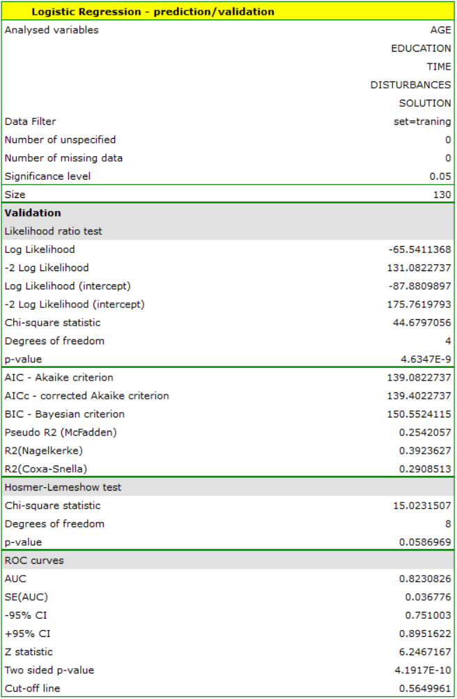
For the training set, the values describing the quality of the model's fit are not very high $Pseudo R^2 = 0.26$ and $R^2(Nagelkerke) = 0.39$ , but already the quality of its prediction is satisfactory (AUC[95%CI]=0.82[0.75, 0.90], sensitivity =82%, specificity 60%).

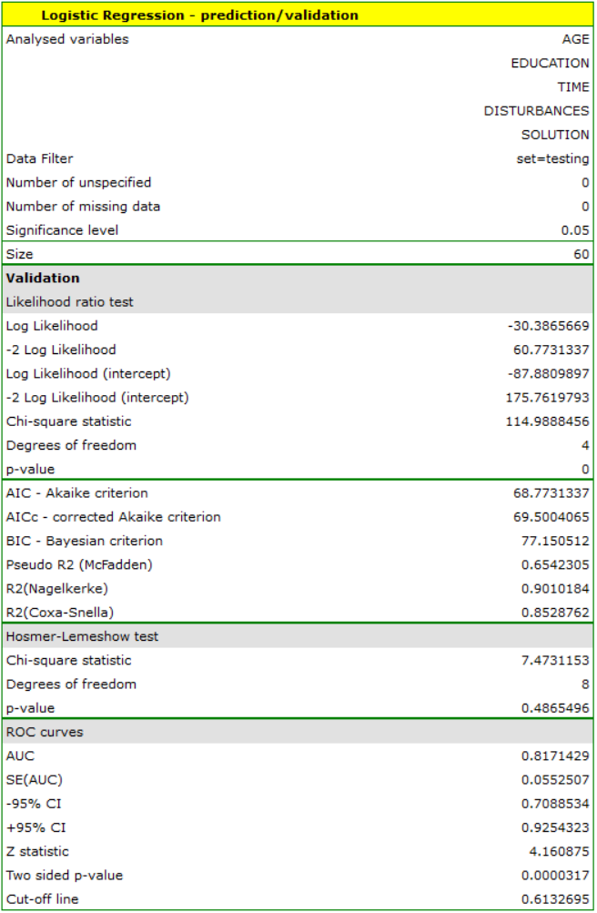
For the test set, the values describing the quality of the model fit are even higher than for the training data $Pseudo R^2 = 0.65$ and $R^2(Nagelkerke) = 0.90$ . The prediction quality for the test data is still satisfactory (AUC[95%CI]=0.82[0.71, 0.93], sensitivity =73%, specificity 64%), so we will use the model for prediction. To do this, we will use the data of three new individuals added at the end of the set. We'll select Prediction, set a filter on the new dataset, and use our model to predict whether the person will solve the task correctly (get a value of 1) or incorrectly (get a value of 0).

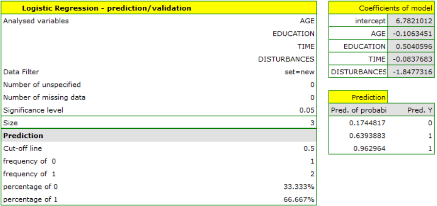
We find that the prediction for the first person is negative, while the prediction for the next two is positive. The prognosis for a 50-year-old woman with an elementary education solving the test during the interference in 20 minutes is 0.17, which means that we predict that she will solve the task incorrectly, while the prognosis for a woman 20 years younger is already favorable - the probability of her solving the task is 0.64. The highest probability (equal to 0.96) of a correct solution has the third woman, who solved the test in 10 minutes and without disturbances.

If we wanted to make a prediction based on another model (e.g., obtained during another scientific study: SOLUTION=6-0.1*AGE+0.5*EDUCATION-0.1*TIME-2*DISTURBANCES) - it would be enough to select a new model in the analysis window, set its coefficients and the forecast for the selected people can be repeated based on this model.

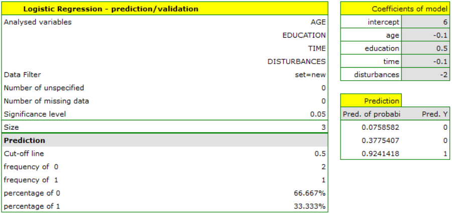
This time, according to the prediction of the new model, the prediction for the first and second person is negative, and the third is positive.

2022/02/09 12:56

Comparison of logistic regression models

The window with settings for model comparison is accessed via the menu Advanced Statistics→Multivariate models→Logistic regression – comparing models

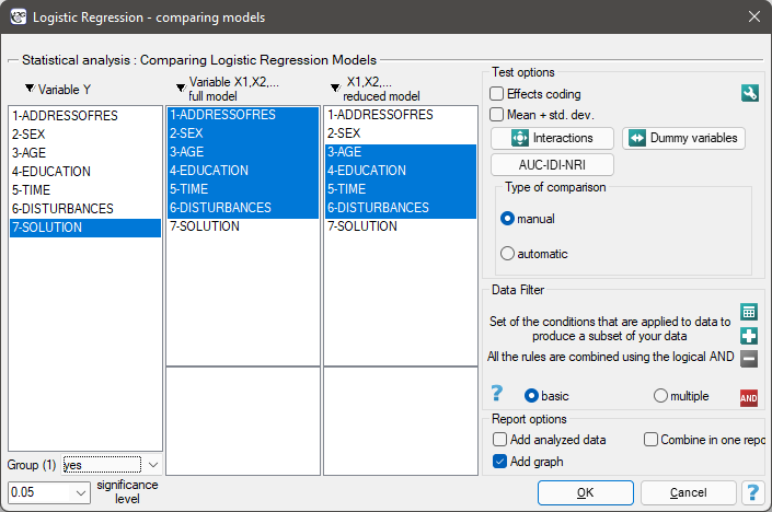
Due to the possibility of simultaneous analysis of many independent variables in one logistic regression model, similarly to the case of multiple linear regression, there is a problem of selection of an optimum model. When choosing independent variables one has to remember to put into the model variables strongly correlated with the dependent variable and weakly correlated with one another.

When comparing models with different numbers of independent variables, we pay attention to model fit and information criteria. For each model we also calculate the maximum of the credibility function, which we then compare using the credibility quotient test.

Hypotheses:

$\begin{array}{cc} \mathcal{H}_0: & L_{FM}=L_{RM},\\ \mathcal{H}_1: & L_{FM}\ne L_{RM}, \end{array}$

where:

$L_{FM}, L_{RM}$ – the maximum of likelihood function in compared models (full and reduced).

The test statistic has the form presented below:

$\begin{displaymath} \chi^2=-2\ln(L_{RM}/L_{FM})=-2\ln(L_{RM})-(-2\ln(L_{FM})) \end{displaymath}$

The statistic asymptotically (for large sizes) has the Chi-square distribution with $df=k_{FM}-k_{RM}$ degrees of freedom, where $k_{FM}$ i $k_{RM}$ is the number of estimated parameters in compared models.

The p-value, designated on the basis of the test statistic, is compared with the significance level $\alpha$ :

$\begin{array}{ccl} $ if $ p \le \alpha & \Longrightarrow & $ reject $ \mathcal{H}_0 $ and accept $ \mathcal{H}_1, \\ $ if $ p > \alpha & \Longrightarrow & $ there is no reason to reject $ \mathcal{H}_0. \\ \end{array}$

We make the decision about which model to choose on the basis of the size $R_{Pseudo}^2$ , $R^2_{Nagelkerke}$ , $R^2_{Cox-Snell}$ and the result of the Likelihood Ratio test which compares the subsequently created (neighboring) models. If the compared models do not differ significantly, we should select the one with a smaller number of variables. This is because a lack of a difference means that the variables present in the full model but absent in the reduced model do not carry significant information. However, if the difference is statistically significant, it means that one of them (the one with the greater number of variables, with a greater $R^2$ and a lower information criterion value of AIC, AICc or BIC) is significantly better than the other one.

Comparison the predictive value of models.

The regression models that are built allow to predict the probability of occurrence of the studied event based on the analyzed independent variables. When many variables (factors) that increase the risk of an event are already known, then an important criterion for a new candidate risk factor is the improvement in prediction performance when that factor is added to the model. To establish the point, let's use an example. Suppose we are studying risk factors for coronary heart disease. Known risk factors for this disease include age, systolic and diastolic blood pressure values, obesity, cholesterol, or smoking. However, the researchers are interested in how much the inclusion of individual factors in the regression model will significantly improve disease risk estimates. Risk factors added to a model will have predictive value if the new and larger model (which includes these factors) shows better predictive value than a model without them. The predictive value of the model is derived from the determined value of the predicted probability of an event, in this case coronary artery disease. This value is determined from the model for each individual tested. The closer the predicted probability is to 1, the more likely the disease is. Based on the predicted probability, the value of the AUC area under the ROC curve can be determined and compared between different models, as well as the $NRI$ and $IDI$ coefficient.

Change of the area under the ROC curve

The ROC curve in logistic regression models is constructed based on the classification of cases into a group experiencing an event or not, and the predicted probability of the dependent variable $P$ . The larger the area under the curve, the more accurately the probability determined by the model predicts the actual occurrence of the event. If we are comparing models built on the basis of a larger or smaller number of predictors, then by comparing the size of the area under the curve we can check whether the addition of factors has significantly improved the prediction of the model.

Hypotheses:

$\begin{array}{cl} \mathcal{H}_0: & AUC_{FM}=AUC_{RM}, \mathcal{H}_1: & AUC_{FM}\neq AUC_{RM}. \end{array}$

For a method of determining the test statistic based on DeLong's method, check out Comparing ROC curves.

The p-value, designated on the basis of the test statistic, is compared with the significance level $\alpha$ :

$\begin{array}{ccl} $ if $ p \le \alpha & \Longrightarrow & $ reject $ \mathcal{H}_0 $ and accept $ \mathcal{H}_1, \\ $ if $ p > \alpha & \Longrightarrow & $ there is no reason to reject $ \mathcal{H}_0. \\ \end{array}$

Net reclassification improvement

This measure is denoted by the acronym $NRI$ The $NRI$ focuses on the reclassification table describing the upward or downward shift in probability values when a new factor is added to the model. It is determined based on two separate factors, i.e., a factor determined separately for subjects experiencing the event (1) and separately for those not experiencing the event (0). The $NRI$ can be determined with a given division of the predicted probability into categories (categorical $NRI$ ) or without the need to determine the categories (continuous $NRI$ ).

NRI categorical requires an arbitrary determination of the division of probability values predicted from the model. There can be a maximum of 9 split points given, and thus a maximum of 10 predicted categories. However, one or two split points are most commonly used. At the same time, it should be noted that the values of the categorical $NRI$ can be compared with each other only if they were based on the same split points. To illustrate the situation, let's establish two example probability split points: 0.1 and 0.3. If a test person in the „old” (smaller) model received a probability below 0.1, and in the „new model” (increased by a new potential risk factor) probability located between 0.1 and 0.3, it means that the person was reclassified upwards (table, situation 1). If the probability values from both models are in the same range, then the person is not reclassified (table, situation 2), whereas if the probability from the „new” model is lower than that from the „old” model, then the person is reclassified downwards (table, situation 3).

$\begin{tabular}{|c|c|c||c|c||c|c|} \hline regression models&\multicolumn{2}{|c||}{situation 1}&\multicolumn{2}{|c||}{situation 2}&\multicolumn{2}{|c|}{situation 3}\\\hline predicted probability&"old"&"new"&"old"&"new"&"old"&"new"\\\hline [0.3 do 1]&&&&&$\oplus$&\\\hline [0.1; 0.3)&&$\oplus$&$\oplus$&$\oplus$&&$\oplus$\\\hline [0; 0.1)&$\oplus$&&&&&\\\hline \end{tabular}$

NRI continuous does not require an arbitrary designation of categories, since any, even the smallest, change in probability up or down from the probability designated in the „old model” is treated as a transition to the next category. Thus, there are infinitely many categories, just as there are many possible changes.

Note

Use of continuous $NRI$ does not require arbitrary definition of probability split points, but even small changes in risk (not reflected in clinical observations) can increase or decrease this ratio. The categorical $NRI$ factor allows only changes that are important to the investigator to reflect changes that involve exceeding preset event risk values (predicted probability values).

To determine $NRI$ we define:

$\hat{p}_{up,events}=\frac{\#events_{up}}{\#events}$

$\hat{p}_{down,events}=\frac{\#events_{down}}{\#events}$

$\hat{p}_{up,nonevents}=\frac{\#nonevents_{up}}{\#nonevents}$

$\hat{p}_{down,nonevents}=\frac{\#nonevents_{down}}{\#nonevents}$

where:

$\#events_{up}$ – the number of subjects in the group experiencing the event for whom there was an upward change of at least one category in the predicted probability,

$\#events_{down}$ – the number of subjects in the group experiencing the event for whom there was at least one downward change in predicted probability,

$\#events$ – number of objects in the group experiencing the event,

$\#nonevents_{up}$ – The number of subjects in the group not experiencing the event for whom there was an upward change of at least one category in the predicted probability,

$\#nonevents_{down}$ – The number of subjects in the group not experiencing the event for whom there was at least one downward change in predicted probability,

$\#nonevents$ – number of objects in the group not experiencing the event.

The overall $NRI$ and coefficients expressing the percentage change in classification are determined from the formula:

$\begin{displaymath} NRI=\left(\hat{p}_{up,events}-\hat{p}_{down,events}\right)-\left(\hat{p}_{up,nonevents}-\hat{p}_{down,nonevents}\right) \end{displaymath}$

$\begin{displaymath} NRI_{events}=\hat{p}_{up,events}-\hat{p}_{down,events}, \quad NRI_{nonevents}=\hat{p}_{down,nonevents}-\hat{p}_{up,nonevents}, \end{displaymath}$

The $NRI_{events}$ coefficient can be interpreted as the net percentage of correctly reclassified individuals with an event, and $NRI_{nonevents}$ as the net percentage of correctly reclassified individuals without an event. The overall coefficient $NRI$ is expressed as the sum of the coefficients $NRI_{events}$ and $NRI_{nonevents}$ making it a coefficient implicitly weighted by event frequency and cannot be interpreted as a percentage.

The $NRI_{events}$ coefficientsbelong to the range from-1 to 1 (from -100% to 100%), and the overall coefficients of $NRI$ belong to the range from -2 to 2. Positive values of the coefficients indicate favorable reclassification, and negative values indicate unfavorable reclassification due to the addition of a new variable to the model.

Z test for significance of NRI coefficient

Using this test, we examine whether the change in classification expressed by the $NRI$ coefficient was significant.

Hypotheses:

$\begin{array}{cl} \mathcal{H}_0: & NRI=0,\\ \mathcal{H}_1: & NRI\neq 0. \end{array}$

The test statistic has the form:

$\begin{displaymath} Z=\frac{NRI}{SE(NRI)} \end{displaymath}$

where:

$\begin{array}{cl} SE(NRI)= & [\left(\frac{\#events_{up} + \#events_{down}}{\#events^2}-\frac{(\#events_{up} + \#events_{down})^2}{\#events^3}\right)+\\ & +\left(\frac{\#nonevents_{down} + \#nonevents_{up}}{\#nonevents^2}-\frac{(\#nonevents_{down} + \#nonevents_{up})^2}{\#nonevents^3}\right)]^{1/2} \end{array}$

The $Z$ statistic asymptotically (for large sample sizes) has the normal distribution.

The p-value, designated on the basis of the test statistic, is compared with the significance level $\alpha$ :

$\begin{array}{ccl} $ if $ p \le \alpha & \Longrightarrow & $ reject $ \mathcal{H}_0 $ and accept $ \mathcal{H}_1, \\ $ if $ p > \alpha & \Longrightarrow & $ there is no reason to reject $ \mathcal{H}_0. \\ \end{array}$

Integrated Discrimination Improvement

This measure is denoted by the abbreviation $IDI$ . The $IDI$ coefficients indicate the difference between the value of the average change in the predicted probability between the group of objects experiencing the event and the group of objects that did not experience the event.

$\begin{displaymath} IDI=\overline{p(diff)}_{events}-\overline{p(diff)}_{nonevents} \end{displaymath}$

where:

$\overline{p(diff)}_{events}$ – The mean of the difference in predicted probability values between the regression models („old” and „new”) for objects that experienced the event,

$\overline{p(diff)}_{nonevents}$ – The mean of the difference in predicted probability values between the regression models („old” and „new”) for objects that did not experience the event.

Z test for significance of IDI coefficient

Using this test, we examine whether the difference between the value of the mean change in predicted probability between the group of subjects experiencing the event and the subjects not experiencing the event, as expressed by the $IDI$ coefficient, was significant.

Hypotheses:

$\begin{array}{cl} \mathcal{H}_0: & IDI=0,\\ \mathcal{H}_1: & IDI\neq 0. \end{array}$

The test statistic is of the form:

$\begin{displaymath} Z=\frac{IDI}{SE(IDI)} \end{displaymath}$

where:

$SE(IDI)=\sqrt{\frac{sd(diff)^2_{events}}{\#events}+\frac{sd(diff)^2_{nonevents}}{\#nonevents}}$

The $Z$ statistic asymptotically (for large sample sizes) has the normal distribution.

The p-value, designated on the basis of the test statistic, is compared with the significance level $\alpha$ :

$\begin{array}{ccl} $ if $ p \le \alpha & \Longrightarrow & $ reject $ \mathcal{H}_0 $ and accept $ \mathcal{H}_1, \\ $ if $ p > \alpha & \Longrightarrow & $ there is no reason to reject $ \mathcal{H}_0. \\ \end{array}$

In the program PQStat the comparison of models can be done manually or automatically.

Manual model comparison – construction of 2 models:
- a full model – a model with a greater number of variables,
- a reduced model – a model with a smaller number of variables – such a model is created from the full model by removing those variables which are superfluous from the perspective of studying a given phenomenon.

The choice of independent variables in the compared models and, subsequently, the choice of a better model on the basis of the results of the comparison, is made by the researcher.

Automatic model comparison is done in several steps:

[step 1] Constructing the model with the use of all variables.
[step 2] Removing one variable from the model. The removed variable is the one which, from the statistical point of view, contributes the least information to the current model.
[step 3] A comparison of the full and the reduced model.
[step 4] Removing another variable from the model. The removed variable is the one which, from the statistical point of view, contributes the least information to the current model.
[step 5] A comparison of the previous and the newly reduced model.
[…]

In that way numerous, ever smaller models are created. The last model only contains 1 independent variable.

EXAMPLE cont. (task.pqs file)

In the experiment made with the purpose to study, for 130 people of the teaching set, the concentration abilities a logistic regression model was constructed on the basis of the following variables:

dependent variable: SOLUTION (yes/no) - information about whether the task was correctly solved or not;

independent variables:

ADDRESSOFRES (1=city/0=village),

SEX (1=female/0=male),

AGE (in years),

EDUCATION (1=primary, 2=vocational, 3=secondary, 4=tertiary),

TIME needed for the completion of the task (in minutes),

DISTURBANCES (1=yes/0=no).

Let us check if all independent variables are indispensible in the model.

Manual model comparison.

On the basis of the previously constructed full model we can suspect that the variables: ADDRESSOFRES and SEX have little influence on the constructed model (i.e. we cannot successfully make classifications on the basis of those variables). Let us check if, from the statistical point of view, the full model is better than the model from which the two variables have been removed.

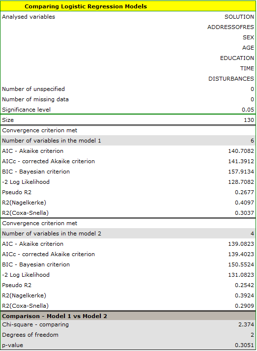
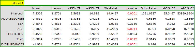
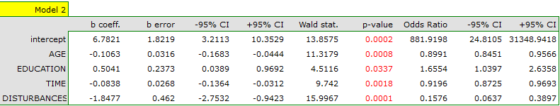
The results of the Likelihood Ratio test ( $p=0.3051$ ) indicates that there is no basis for believing that a full model is better than a reduced one. Therefore, with a slight worsening of model adequacy, the address of residence and the sex can be omitted.

We can compare the two models in terms of classification ability by comparing the ROC curves for these models, NRI and IDI value. To do so, we select the appropriate option in the analysis window. The resulting report, like the previous one, indicates that the models do not differ in prediction quality i.e. the p-values for the comparison of ROC curves and for the evaluation of NRI and IDI indices are statistically insignificant. We therefore decide to omit gender and place of residence from the final model.

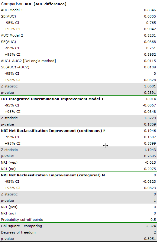
Automatic model comparison.

For automatic model comparison, we obtained very similar results. The best model is the model built on the independent variables: AGE, EDUCATION, TIME OF SOLUTION, and DISTURBANCES. Based on the above analyses, from a statistical point of view, the optimal model is one containing the 4 most important independent variables: AGE, EDUCATION, RESOLUTION TIME, and DISTURBANCES. Its detailed analysis can be done in the Logistic Regression module. However, the final decision which model to choose is up to the experimenter.

EXAMPLE (Heart.pqs file)

Risk factors for certain heart disease such as age, bmi, smoking, LDL fraction cholesterol, HDL fraction cholesterol, and hypertension were examined. From the researcher's point of view, it was interesting to determine how much information about smoking could improve the prediction of the occurrence of the disease under study.

We compare a logistic regression model describing the risk of heart disease based on all study variables with a model without smoking information. In the analysis window, we select the options related to the prediction evaluation, namely the ROC curve and the NRI coefficients. In addition, we indicate to include all proposed graphs in the report.

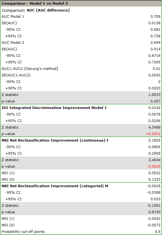
Analysis of the report indicates important differences in prediction as a result of adding smoking information to the model, although they are not significant in describing the ROC curve (p=0.057).

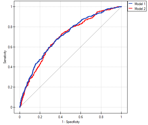
The continuous IDI and NRI coefficient values indicate a statistically significant and favorable change (the values of these coefficients are positive with p<0.05). The prognosis for those with heart disease improved by more than 5% and those without heart disease by more than 13% (NRI(sick)=0.0522, NRI(healthy)=0.1333)) as a result of including information about smoking.

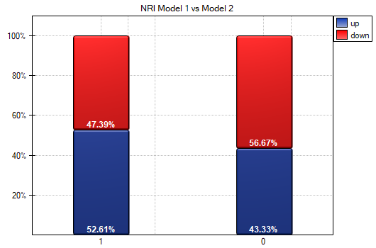
We also see the conclusions drawn from the NRI in the graph. We see an increase in the model-predicted probability of disease in diseased individuals (more individuals were reclassified upward than downward 52.61% vs 47.39%) while a decrease in the probability applies more to healthy individuals (more individuals were reclassified downward than upward 56.67% vs 43.33%). It is also possible to determine a categorical NRI, but to do so, one would first need to determine the model-determined probability cut-off points accepted in the heart disease literature.

2022/02/09 12:56

Factorial ANOVA - GLM

Okno z ustawieniami opcji ANOVA czynnikowa GLM wywołujemy poprzez menu Statystyka→Modele wielowymiarowe→ANOVA czynnikowa GLM

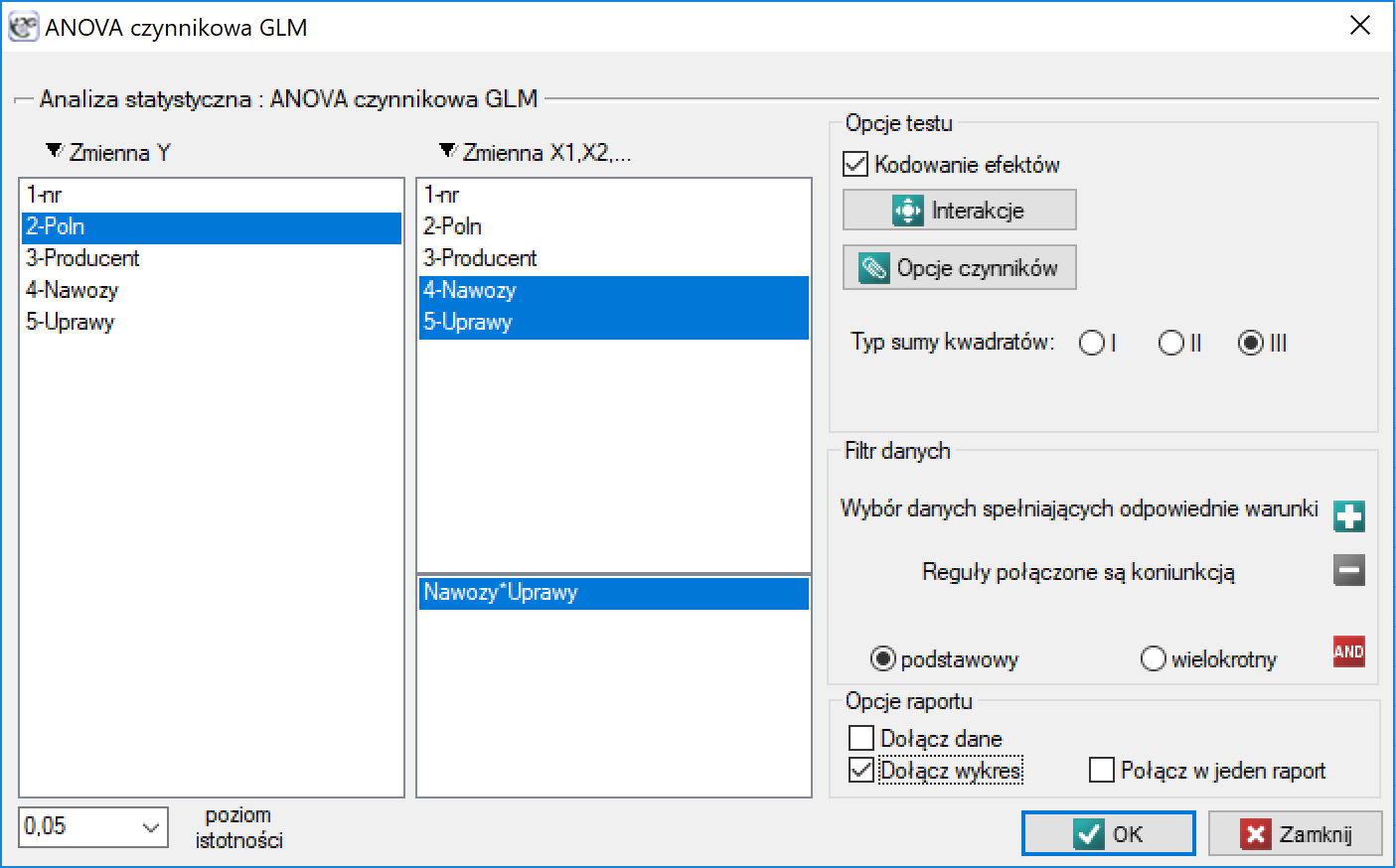
Czynnikowa analiza wariancji GLM jest rozszerzeniem jednoczynnikowej analizy wariancji (ANOVA) dla grup niezależnych oraz liniowej regresji wielorakiej. Skrót GLM (ang. general linear model) czytamy jako Ogólny Model Liniowy. Analiza GLM polega zwykle na wykorzystaniu modeli regresji liniowej w wyliczaniu różnych złożonych porównań ANOVA.

Przykład

Przykład równoważnych analiz, które mogą być przeprowadzone poprzez GLM. Analizy zawarte w poszczególnych wierszach tabeli są równoważne w tym sensie, że ich wyniki są tożsame, choć nie muszą być identyczne.

Badanie dotyczy dochodu pewnej grupy osób. O badanych osobach mamy pewne dodatkowe informacje typu: płeć i wykształcenie.

$\begin{tabular}{|c|l|l|} \hline dochód oraz...&ANOVA&Regresja wieloraka \\\hline &\footnotesize \textbf{t-studenta dla zmiennych niezależnych} &\footnotesize \textbf{zależność dochodu ($Y$) od płci ($X$)}\\ \footnotesize płeć &\footnotesize $\star$ porównanie dochodu dla kobiet z dochodem dla mężczyzn &\footnotesize $\star$ płeć jako kolumna o dwóch kategoriach\\\hline &\footnotesize \textbf{ANOVA jednoczynnikowa} &\footnotesize \textbf{zależność dochodu ($Y$) od wykształcenia ($X$)}\\ \footnotesize wykształcenie &\footnotesize $\star$ porównanie dochodu dla osób z różnym wykształceniem &\footnotesize $\star$ wykształcenie rozbite na zmienne fikcyjne\\ &\footnotesize (podstawowym, zawodowym, średnim, wyższym) & \\\hline &\footnotesize \textbf{ANOVA wieloczynnikowa} &\footnotesize \textbf{zależność dochodu ($Y$) od płci ($X_1$)}\\ \footnotesize płeć, &\footnotesize $\star$ porównanie dochodu dla kobiet z dochodem dla mężczyzn &\footnotesize \textbf{i wykształcenia ($X_2$)}\\ &\footnotesize przy uwzględnieniu wykształcenia jako zmiennej wikłającej &\footnotesize $\star$ płeć jako kolumna o dwóch kategoriach\\ \footnotesize wykształcenie &\footnotesize $\star$ porównanie dochodu dla osób z różnym wykształceniem &\footnotesize $\star$ wykształcenie rozbite na zmienne fikcyjne\\ &\footnotesize (podstawowym, zawodowym, średnim, wyższym) &\\ &\footnotesize przy uwzględnieniu płci jako zmiennej wikłającej &\footnotesize obie zmienne są wzajemnie wikłające\\\hline &\footnotesize \textbf{ANOVA wieloczynnikowa} &\footnotesize \textbf{zależność dochodu ($Y$) od płci ($X_1$), }\\ \footnotesize płeć, &\footnotesize $\star$ porównanie dochodu dla kobiet z dochodem dla mężczyzn &\footnotesize \textbf{od wykształcenia ($X_2$) oraz od}\\ &\footnotesize przy uwzględnieniu innych zmiennych w modelu &\footnotesize \textbf{interakcji płci i wykształcenia ($X_1*X_2$)}\\ \footnotesize wykształcenie, &\footnotesize $\star$ porównanie dochodu dla osób z różnym wykształceniem &\footnotesize $\star$ płeć jako kolumna o dwóch kategoriach\\ &\footnotesize (podstawowym, zawodowym, średnim, wyższym) &\footnotesize $\star$ wykształcenie rozbite na zmienne fikcyjne\\ &\footnotesize przy uwzględnieniu innych zmiennych w modelu &\footnotesize $\star$ interakcja to iloczyn płci i wykształcenia\\ \footnotesize płeć*wykształcenie &\footnotesize $\star$ porównanie dochodu dla osób z różnym & \\ &\footnotesize wykształceniem i płcią (w interakcji)&\footnotesize zmienne w modelu są wzajemnie wikłające\\ &\footnotesize przy uwzględnieniu innych zmiennych w modelu &\\\hline \end{tabular}$

Analiza GLM może być wykorzystana w każdym z powyższych przypadków, ponieważ jednak analiza regresji wielorakiej podobnie jak jednoczynnikowa ANOVA zostały omówione w oddzielnych rozdziałach, w tym rozdziale przedstawimy wykorzystanie GLM w ANOVA wieloczynnikowa.

ANOVA czynnikowa jest takim rodzajem analizy wariancji, w którym możemy wykorzystać zarówno jedną jak i wiele czynników by wyodrębnić porównywane grupy. W analizie mogą brać udział również takie zmienne, które są interakcją wskazanych czynników. Gdy ANOVA zawiera więcej czynników niż jeden, wówczas czynniki te są wobec siebie uwikłane.

Wpływ czynników wikłających

Pomimo, że wszystkie czynniki biorące udział w analizie są wobec siebie uwikłane, to ich wpływ na istotność poszczególnych czynników można kontrolować. Istnieją trzy sposoby, przy pomocy których badając istotność poszczególnych czynników można uwzględniać wpływ zmiennych wikłających. Zależą one od sposobu wyznaczania sumy kwadratów:

Sumy kwadratów typu I

Sumy kwadratów typu I zależą od kolejności w jakiej w modelu znajdują się poszczególne czynniki. Ten rodzaj sumy kwadratów powoduje, że istotność czynnika który interpretujemy jest korygowana o te zmienne, których kolejność w modelu była wcześniejsza, pozostałe zmienne w modelu wpływają jedynie pośrednio na wynik analizy. Na przykład: jeśli w modelu umieszczamy czynniki we wskazanej kolejności: $A$ , $B$ , $A*B$ , $C$ , $A*C$ , $B*C$ , $A*B*C$ , $D$ , wówczas istotność dla czynnika $A*C$ uwzględnia cały model (poprzez sumy kwadratów dla błędu) ale jako zmienne wikłające wykorzystywane są wprost tylko czynniki: $A$ , $B$ , $A*B$ , $C$ .

Sumy kwadratów dla czynnika $A*C$ wylicza się wówczas następująco: $\begin{displaymath} SS(A*C)=SS(A, B, A*B, C, A*C, B*C, A*B*C, D)-SS(A, B, A*B, C) \end{displaymath}$

Stosowanie sumy kwadratów typu I

Wskazania: Kiedy badanie jest w pełni zbalansowane, z równymi lub proporcjonalnymi licznościami poszczególnych kategorii, również wtedy, gdy występują interakcje.

Przeciwwskazania: Kiedy badanie jest niezbalansowane (różne liczności poszczególnych kategorii) i/lub występują interakcje.

Sumy kwadratów typu II

Ten rodzaj sumy kwadratów powoduje, że istotność czynnika który interpretujemy jest korygowana o te zmienne, których rząd jest taki sam lub niższy, pozostałe zmienne w modelu wpływają jedynie pośrednio na wynik analizy. Na przykład: jeśli w modelu umieszczamy czynniki: $A$ , $B$ , $A*B$ , $C$ , $A*C$ , $B*C$ , $A*B*C$ , $D$ , wówczas istotność dla czynnika $A*C$ uwzględnia cały model (poprzez sumy kwadratów dla błędu) ale jako zmienne wikłające wykorzystywane są wprost zmienne pierwszego rzędu: $A$ , $B$ , $C$ , $D$ oraz wszystkie pozostałe zmienne drugiego rzędu: $A*B$ , $B*C$ .

Sumy kwadratów dla czynnika $A*C$ wylicza się wówczas następująco: $\begin{displaymath} SS(A*C)=SS(A, B, A*B, C, A*C, B*C, A*B*C, D)-SS(A, B, A*B, C, B*C, D) \end{displaymath}$

Stosowanie sumy kwadratów typu II

Wskazania: Kiedy badanie jest w pełni zbalansowane, z równymi lub proporcjonalnymi licznościami poszczególnych kategorii, również wtedy, gdy występują interakcje.

Przeciwwskazania: Kiedy badanie jest niezbalansowane (różne liczności poszczególnych kategorii) i/lub występują interakcje.

Sumy kwadratów typu III

Zalecamy stosować ten rodzaj kodowania, gdy wybrane jest kodowanie efektów.

Ten rodzaj sumy kwadratów powoduje, że istotność czynnika który interpretujemy jest korygowana o wszystkie pozostałe zmienne w modelu. Na przykład: jeśli w modelu umieszczamy czynniki: $A$ , $B$ , $A*B$ , $C$ , $A*C$ , $B*C$ , $A*B*C$ , $D$ , wówczas istotność dla zmiennej $A*C$ uwzględnia cały model (poprzez sumy kwadratów dla błędu) a jako zmienne wikłające wykorzystywane są wprost wszystkie czynniki za wyjątkiem badanego: $A$ , $B$ , $A*B$ , $C$ , $B*C$ , $A*B*C$ , $D$ ,.

Sumy kwadratów dla czynnika $A*C$ wylicza się wówczas następująco: $\begin{displaymath} SS(A*C)=SS(A, B, A*B, C, A*C, B*C, A*B*C, D)-SS(A, B, A*B, C, B*C, A*B*C, D) \end{displaymath}$

Stosowanie sumy kwadratów typu III

Wskazania: Kiedy badanie jest zbalansowane lub niezbalansowane, również wtedy, gdy występują interakcje.

Przeciwwskazania: Kiedy badanie zawiera podklasy o brakujących obserwacjach.

W PQStat domyślnie wybrane są sumy kwadratów typu III, ze względu na ich uniwersalność. Domyślnie zaznaczona jest też opcja kodowanie efektów opisana w rozdziale Przygotowanie zmiennych do analizy. Należy pamiętać, że wybór odpowiedniego kodowania wpływa zarówno na interpretację współrzędnych modelu jak i na istotność poszczególnych czynników w ANOVA czynnikowa - szczególnie przy niezbalansowanych układach.

Podstawowe warunki stosowania:

pomiar na skali interwałowej,
próby pochodzą z populacji o rozkładzie normalnym normalność zmiennych bądź reszt modelu),
model niezależny,
równość wariancji badanych zmiennych porównywanych populacji.

ANOVA czynnikowa wymaga by czynniki dzieliły się na poszczególne kategorie (tj. niezależne populacje) np. czynnik $A$ : płeć dzielimy na męską i żeńską, czynnik $B$ : wykształcenie na podstawowe, zawodowe, średnie i wyższe. Interakcja czynnika $A*B$ jest również dzielona na kategorie, w tym przypadku kategorii uzyskamy osiem:

1) kategoria żeńska z wykształceniem podstawowym,

2) żeńska z wykształceniem zawodowym,

3) żeńska z wykształceniem średnim,

4) żeńska z wykształceniem wyższym,

5) kategoria męska z wykształcniem podstawowym,

6) męska z wykształceniem zawodowym,

7) męska z wykształceniem średnim,

8) męska z wykształceniem wyższym.

Analiza typu ANOVA i modele regresji traktowane są równoważnie, i w ogólnym przypadku ich hipotezy są zbieżne. Hipotezy dla efektów głównych $A$ i $B$ i efektu interakcji $A*B$ przedstawimy w obu tych ujęciach. W interpretacji tych hipotez należy pamiętać, że hipotezy dla danych czynników korygowane są o te z pozostałych czynników, które dana analiza uwzględnia.

Podejście ANOVA

Hipotezy dla czynnika $A$ :

$\begin{array}{cl} \mathcal{H}_0: & \mu_1=\mu_2=...=\mu_a,\\ \mathcal{H}_1: & $nie wszystkie $\mu_i$ są sobie równe $(i=1,2,...,a)$$, \end{array}$

gdzie:

$\mu_1$ , $\mu_2$ ,…, $\mu_a$ $-$ średnie czynnika $A$ dla poszczególnych jego kategorii.

Hipotezy dla czynnika $B$ :

$\begin{array}{cl} \mathcal{H}_0: & \mu_1=\mu_2=...=\mu_b,\\ \mathcal{H}_1: & $nie wszystkie $\mu_j$ są sobie równe $(j=1,2,...,b)$$, \end{array}$

gdzie:

$\mu_1$ , $\mu_2$ ,…, $\mu_b$ $-$ średnie czynnika $B$ dla poszczególnych jego kategorii.

Hipotezy dla interakcji czynników $A*B$ :

$\begin{array}{cl} \mathcal{H}_0: & \mu_1=\mu_2=...=\mu_{ab},\\ \mathcal{H}_1: & $nie wszystkie $\mu_k$ są sobie równe $(k=1,2,...,ab)$$, \end{array}$

gdzie:

$\mu_1$ , $\mu_2$ ,…, $\mu_{ab}$ $-$ średnie interakcji czynników $A*B$ dla poszczególnych ich kategorii.

Podejście regresyjne

Podejście modelowe zakłada działanie modelu regresji $\begin{displaymath} Y=\mu+\alpha_iA_i+\beta_jB_j+(\alpha\beta)_kB_k+\epsilon. \end{displaymath}$

gdzie:

$Y$ - zmienna zależna, objaśniana przez model,

$\mu$ - średnia ogólna zmiennej $Y$ (o ile zastosowano kodowanie efektów)

$A_i, B_j, AB_k$ - czynniki - zmienne niezależne, objaśniające,

$\alpha_i,\beta_i,\alpha\beta_i,$ - parametry,

$\epsilon$ - składnik losowy (reszta modelu).

Hipotezy dla czynnika $A$ :

$\begin{array}{cl} \mathcal{H}_0: & \alpha_1=\alpha_2=...=\alpha_a=0,\\ \mathcal{H}_1: & $nie wszystkie $\alpha_i=0$$, \end{array}$

Hipotezy dla czynnika $B$ :

$\begin{array}{cl} \mathcal{H}_0: & \beta_1=\beta_2=...=\beta_b=0,\\ \mathcal{H}_1: & $nie wszystkie $\beta_j=0$ $, \end{array}$

Hipotezy dla interakcji czynników $A*B$ :

$\begin{array}{cl} \mathcal{H}_0: & (\alpha\beta)_1=(\alpha\beta)_2=...=(\alpha\beta)_{ab}=0,\\ \mathcal{H}_1: & $nie wszystkie $(\alpha\beta)_k=0$$, \end{array}$

Kodowanie

Uzyskiwane wyniki analiz (w szczególności budowanego modelu regresji) oraz interpretacja hipotez zależą również od sposobu kodowania. Program PQStat oferuje kodowanie zero-jedynkowe i kodowanie efektów. Dokładny opis kodowania można znaleźć w rozdziale Przygotowanie zmiennych do analizy w modelach wielowymiarowych. Domyślnie program wybiera kodowanie efektów. Odznaczenie tej opcji jest równoważne z wybraniem kodowania zero-jedynkowego.

Uwaga!

W przypadku stosowaniu sumy kwadratów typu III, gdy występują interakcje, wskazane jest stosowanie kodowania efektów.

Przykład (plik plon.pqs)

Aby zwiększyć plon roślin uprawnych, opracowuje się nawozy według coraz nowszych technologii. Na podstawie przeprowadzonego eksperymentu badacze chcą się dowiedzieć, która z trzech mieszanek nowych nawozów jest najbardziej skuteczna. Uprawy były prowadzone przez dwa różne gospodarstwa rolne i dotyczyły zasiewu pszenicy, żyta, owsa i jęczmienia. Plon podawano w % (w porównaniu do plonu uzyskanego bez nawożenia).

W pierwszej kolejności chcemy sprawdzić czy:

1) H0: Średnie plony uzyskane przy zastosowaniu nawożenia mieszanką X są takie same jak uzyskane przy nawożeniu mieszanką Y i takie same jak przy nawożeniu mieszanką Z (niezależnie od gospodarstwa prowadzącego uprawę).

Ponadto, choć jest to w tym przypadku miej interesujące, sprawdzimy czy:

2) H0: Średnie plony uzyskane w gospodarstwie 1 są takie same jak w gospodarstwie drugim (niezależnie od mieszanki stosowanego nawozu).

Równoważnie hipotezy te można zapisać korzystając z podejścia regresyjnego:

1) H0: Współczynniki określające zmianę uzyskanego plonu przy zmianie stosowanego nawożenia są zerowe (niezależnie od gospodarstwa prowadzącego uprawę).

2) H0: Współczynnik określający zmianę uzyskanego plonu przy zmianie gospodarstwa prowadzącego uprawę jest zerowy (niezależnie od mieszanki stosowanego nawozu).

W drugiej kolejności stosując GLM sprawdzimy czy:

3) H0: Średnie plony uzyskane z uprawy poszczególnych zbóż są takie same gdy stosujemy różny sposób nawożenia.

Hipotezy 1) i 2)

Podejście ANOVA

Analizę przeprowadzimy stosując trzeci typ sumy kwadratów i kodowanie efektów.

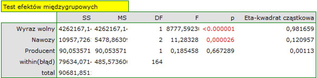
Obserwujemy istotne statystycznie różnice pomiędzy plonem uzyskanym przy zastosowaniu różnych mieszanek nawozów (p=0.000026). Zastosowana mieszanka nawozów tłumaczy zmienność w uzyskanym plonie w około 12% o czym świadczy wartość cząstkowej Eta-kwadrat. Uzyskane plony nie zależą natomiast od tego w jakim gospodarstwie prowadzono uprawy (p=0.667289, Eta-kwadrat cząstkowe = 0,1%).

Po wybraniu średnich obserwowanych lub oczekiwanych w oknie Opcji czynników, różnice te możemy przedstawić graficznie na wykresach obrazujących średnie plony przy stosowaniu poszczególnych mieszanek nawozów. Dokładne wartości średnich możemy odczytać z tabeli statystyk opisowych.

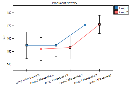
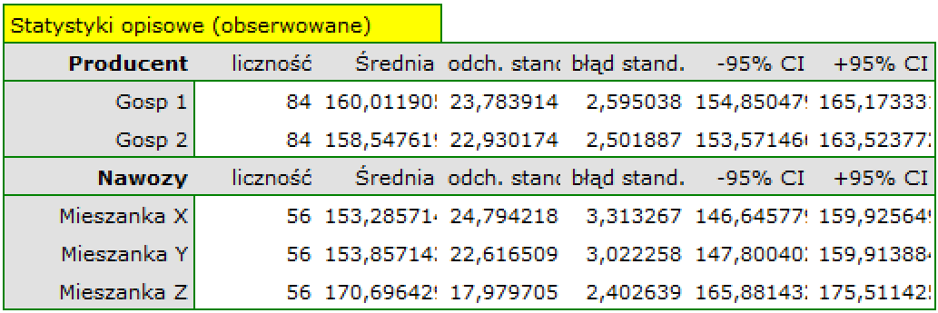
To, gdzie różnice są zlokalizowane możemy sprawdzić stosując testy post-hoc. Test post-hoc NIR Fishera wskazuje, iż najkorzystniejsze rezultaty przynosi stosowanie mieszanki Z – uzyskany plony stanowi średnio 170,7% plonu, który uzyskano by nie stosując nawożenia. Pozostałe mieszani nie różnią się istotnie statystycznie wielkością uzyskanego plonu. Ponieważ w modelu jednoczesnej analizie poddawano gospodarstwo w którym prowadzone były uprawy, możemy powiedzieć, że przewaga mieszanki Z jest niezależna od tego, w którym gospodarstwie wykonano zasiew.

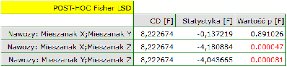
Podejście regresyjne

Analogiczną interpretację uzyskamy posługując się modelem regresji, choć tutaj interpretacja jest nieco trudniejsza. Trudność wynika z konieczności ustalenia sposobu kodowania i wyboru kategorii odniesienia. Przyjrzyjmy się najpierw wynikom otrzymanym przy kodowaniu zero-jedynkowym, które możemy uzyskać odznaczając opcję kodowania efektów. Analiza automatycznie przyjęła alfabetycznie pierwszy poziom jako poziom odniesienia. Dla nawozów poziomem tym była mieszanka X, dla gospodarstw było to gospodarstwo 1.

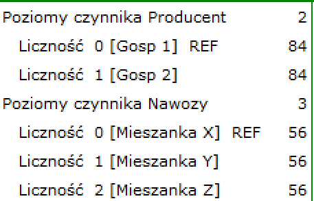
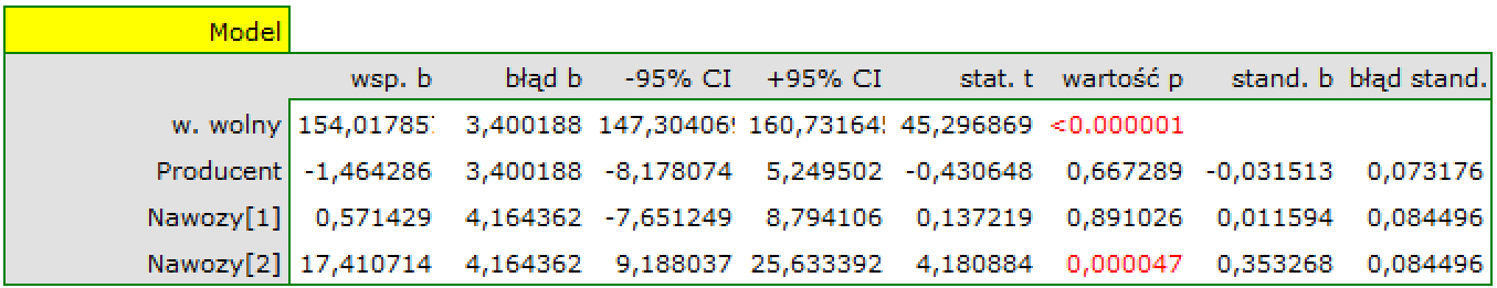
Analiza współczynników modelu przypomina analizę testów post-hoc, z tą różnicą, że porównujemy wyłącznie do kategorii odniesienia. Jeśli więc wszystkie mieszanki nawozów porównamy do mieszanki X możemy zauważyć, że jedynie stosując mieszankę Z uzyskano istotnie wyższe wyniki (p= 0.000047). Wyniki te są wyższe o 17.410714 (przypominam, że średnie wynosiły odpowiednio (153.285714 – dla mieszanki X, 170.696429 – dla mieszanki Z). Porównując gospodarstwa sprawa jest prosta, gdyż mamy do porównania tylko dwa gospodarstwa i uzyskany wynik jest wynikiem porównania gospodarstwa 2 z gospodarstwem 1, które to stanowiło kategorię odniesienia. Tym razem uzyskana różnica była niewielka (-1.464286) i nieistotna statystycznie (0.667289).

Stosując kodowanie efektów również wybieramy kategorię odniesienia, ale wielkość współczynników i ich istotność nie jest odnoszona do wybranej kategorii odniesienia ale do średniej ogólnej uzyskanego plonu, zapisanej w modelu jako wyraz wolny (159.279762).

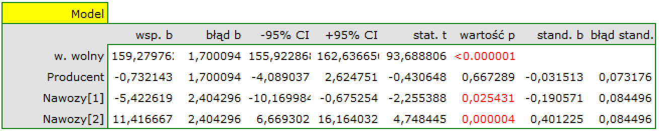
W porównaniu do średniej ogólnej znajdujemy sporo różnic: plon uzyskany przy nawożeniu mieszanką Y jest o 5.422619 niższy niż średnia ogólna, a mieszanką Z o 11.416667 wyższy. Obie różnice są istotne statystycznie.

Niepodważalną zaletą budowania modelu regresyjnego jest możliwość wykorzystania jego formuły w przewidywaniu uzyskanych plonów. Zbudowane modele prezentują się następująco:

Dla kodowania zero-jedynkowego:

$plon=154.017857 + 0.571429\cdot mieszankaY + 17.410714\cdot mieszankaZ - 1.464286\cdot gosp2$

Dla kodowania efektów:

$plon=159.279762 - 5.422619\cdot mieszankaY + 11.416667 \cdot mieszankaZ - 0.732143 \cdot gosp2$

By móc zastosować wybrany model w prognozowaniu należy udać się do menu regresja wieloraka – predykcja i na podstawie nowych danych dokonać predykcji. Przy czym przygotowanie danych zależy od sposobu ich kodowania.

Na podstawie wszystkich uzyskanych wyników nie podejrzewamy by wielkość plonu była zależna od interakcji między rodzajami stosowanych nawozów a gospodarstwem prowadzącym uprawy. Najczęściej występowanie interakcji widoczne jest na wykresie w postaci wyraźnie przecinających się linii. Tu obie linie były prawie równoległe i na tyle bliskie sobie, że różnica między gospodarstwami była nieistotna statystycznie. Mimo, że przecinające się linie najczęściej świadczą o występowaniu interakcji należy pamiętać, żę gdy linie znajdują się blisko siebie ich przypadkowe przecięcie jest bardzo prawdopodobne, w efekcie tego interakcja nie będzie istotna statystycznie. Dla pewności sprawdzimy jednak, czy w naszym przypadku występuje interakcja. W tym celu obie zmienne wybierzemy raz jeszcze w oknie interakcji i przeniesiemy do listy interakcji umieszczonej po prawej stronie okna a następnie powtórzymy analizę.

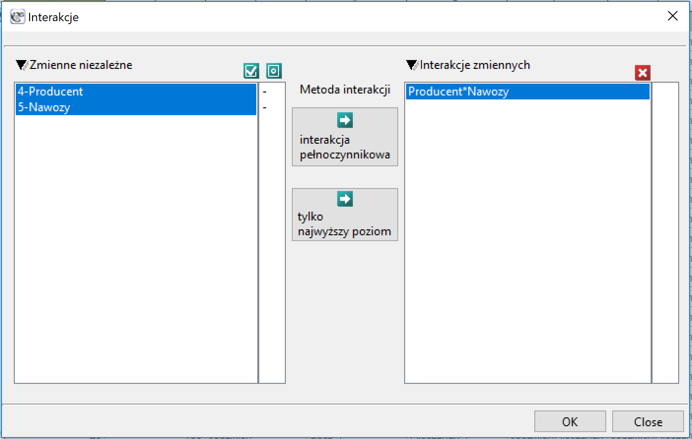
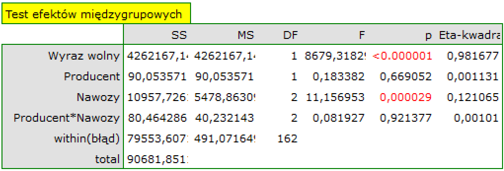
Uzyskany wynik potwierdził nasze przypuszczenia o braku istotnej interakcji (p=0.921377). W tym wypadku zaleca się więc stosowanie modelu prostszego, tzn. pozbawionego interakcji.

Hipoteza 3)

Z odmienną sytuacją zetkniemy się badając wielkość uzyskanego plonu w zależności od stosowanej dawki nawozu oraz w zależności od rodzaju uprawianego zboża.

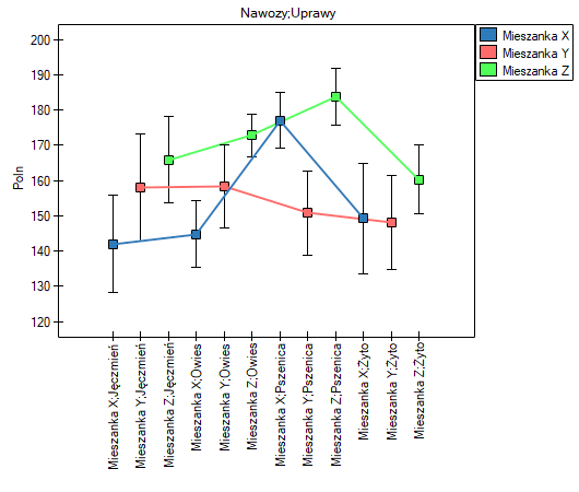
Wykonamy analizę która oprócz efektów głównych uwzględnia interakcje.

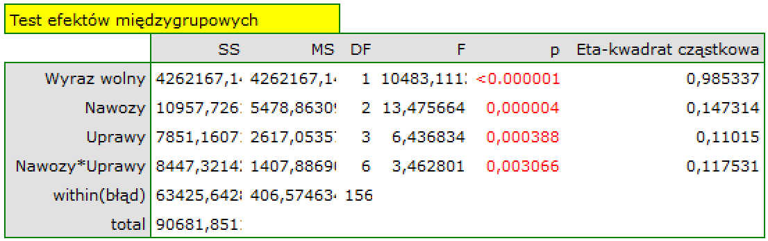
Ponieważ interakcje w zbudowanym modelu są istotne statystycznie (p=0.003066), to właśnie model z interakcjami powinniśmy stosować i opis uzyskanych wyników skupić właśnie na tej interakcji.

W podejściu ANOVA hipoteza odnosząca się do interakcji dotyczy wszystkich możliwych par średnich, tzn.:
H0: Średnie plony uzyskane przy nawożeniu pszenicy mieszanką X są takie same jak przy nawożeniu pszenicy mieszanką Y i takie same jak przy nawożeniu pszenicy mieszanką Z i takie same jak przy nawożeniu żyta mieszanką X i takie same jak przy nawożeniu żyta mieszanką Y i takie same jak przy nawożeniu żyta mieszanką Z i takie same jak przy nawożeniu owsa mieszanką X i takie same jak przy nawożeniu owsa mieszanką Y i takie same jak przy nawożeniu owsa mieszanką Z i takie same jak przy nawożeniu jęczmienia mieszanką X i takie same jak przy nawożeniu jęczmienia mieszanką Y i takie same jak przy nawożeniu jęczmienia mieszanką Z.

W podejściu regresyjnym powiemy, że: H0: Współczynniki określające zmianę uzyskanego plonu przy zmianie stosowanego nawożenia i zmianie rodzaju uprawy są zerowe.
Na podstawie wykresu (oraz średnich zapisanych w tabeli) widzimy iż zdecydowanie najlepsze plony przynosi mieszanka Z, niezależnie od rodzaju uprawianego zboża.

Natomiast mieszanka X i mieszanka Y uzyskują gorsze plony od mieszanki Z i dodatkowo zachodzi między nimi efekt interakcji. Przejawia się ona tym, że uprawa pszenicy przynosi nietypowo wysoki plon w przypadku zastosowania mieszanki X w porównaniu do plonu pszenicy uzyskanego przy nawożeniu Y, podczas gdy uprawa jęczmienia i owsa lepiej plonują, gdy stosowana jest mieszanka Y. Dokładniej uzyskane różnice możemy sprawdzić wykonując testy post-hoc. Fragment tego raportu zamieszczono poniżej:

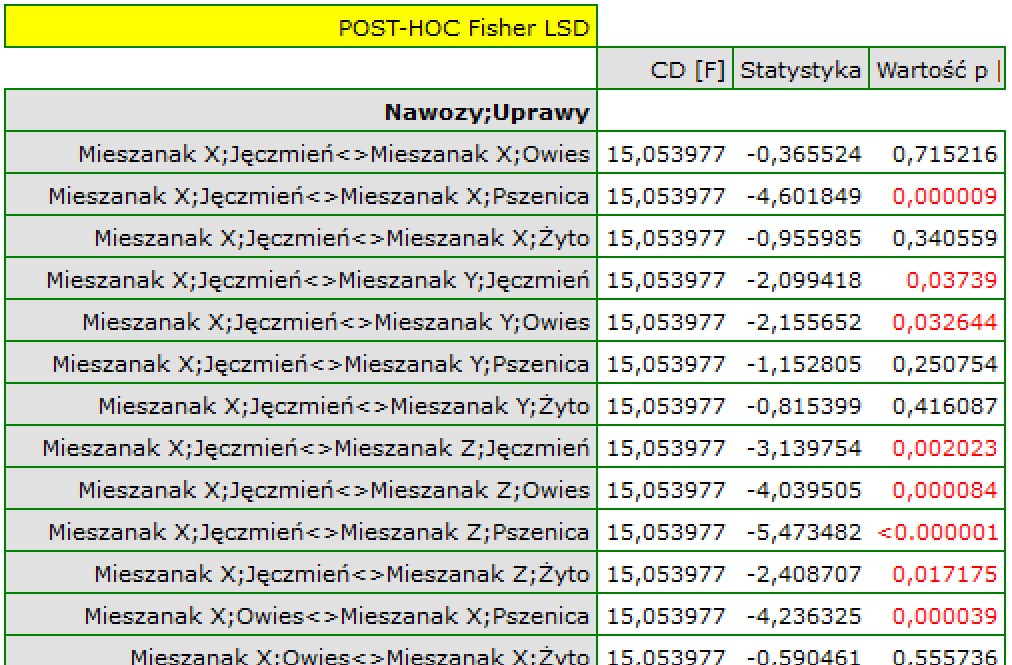
Wynik testu post-hoc Fishera jest obszerny i potwierdza dużą i istotną statystycznie przewagę uzyskanego plonu przy stosowaniu mieszanki Z dla dowolnych upraw i mieszanki Y dla uprawy pszenicy.

Współczynniki modelu regresji możemy wykorzystać do prognozy poprzez menu regresja wieloraka – predykcja pamiętając, by w zależności od wybranego modelu odpowiednio zakodować nowe dane.

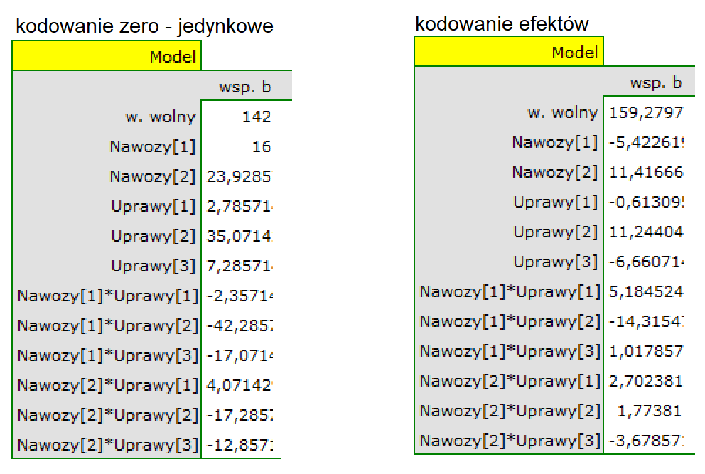
SPRAWDZENIE ZAŁOŻEŃ

Sprawdzenie głównych założeń będzie polegało na porównaniu wariacji oraz wizualnym określeniu normalności reszt modelu.

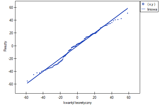
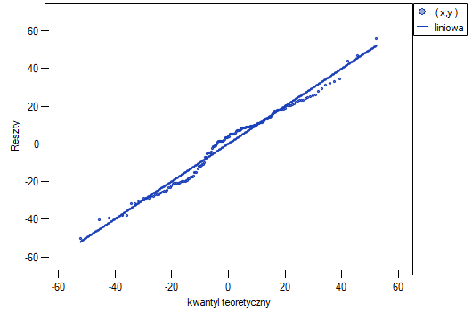
Wykres normalności reszt modelu typu Q-Q dla pierwszej oraz dla drugiej analizy przedstawia reszty modelu dobrze rozlokowane wokół prostej, co świadczy o dobrym dopasowaniu reszt do rozkładu normalnego. Porównaniu wariancji służy test Levenea lub Browna-Forsythea. W przypadku tych testów możemy założyć, że uzyskane wyniki nie są jednoznaczne i są na pograniczu równości wariancji.

2022/02/09 12:56

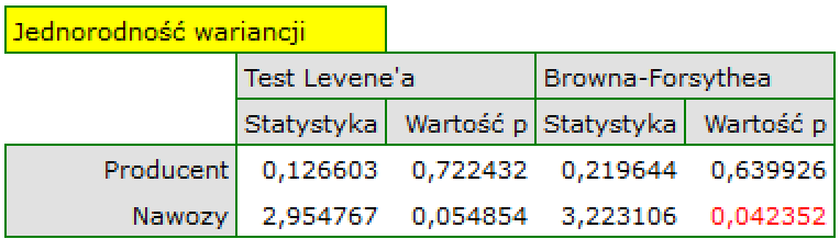
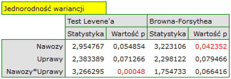
ANCOVA

Analysis of covariance (ANCOVA) is a method of testing the hypothesis that the means of two or more populations are equal, in correction for other continuous variables. These adjustments result in effects more readily seen by researchers than those obtained through ANOVA, i.e., narrower confidence intervals and greater statistical power. Suppose an experiment is conducted to evaluate the effects of two treatments. The groups randomly assigned to treatment differ slightly in mean age, which also affects the treatment effect. Differences between groups in achievement will be quite ambiguous to interpret, since the groups differ in both age and treatment conditions. Analysis of covariance will provide „adjusted averages”, which estimate what the mean scores would be if the groups were exactly the same in terms of age. At the same time, the within-group variability of the results due to the variable (age) will be removed from the error variability to increase the precision of the test of the differences between the adjusted averages.
The label „analysis of covariance” is now seen as anachronistic by some research methodologists and statisticians, since this analysis is not a separate analysis but a variant of the general linear model (GLM). However, the term is still useful because it immediately conveys to most researchers the notion that a categorical variable (e.g., treatment conditions) and a continuous variable (e.g., age) are involved in a single analysis that determines treatment outcome.

The settings window with the ANCOVA can be opened in Advanced statistics→Multivariate models→ANCOVA

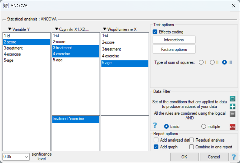
Note!!!

How to take into account the study factors and confounding variables is described in the section on multivariate ANOVA (Influence of confounding factors). The recommended way is to choose Sum of Squares type III and effects coding.

Basic application conditions:

measurement on an interval scale,
the samples come from a population with a normal distribution (normality of the variables or residuals of the model),
an independent model,
equality of variances of an analysed variable in all populations,
Equality of the slopes of the regression lines (regression coefficients between each confounding variable and the dependent variable) for each possible factor level.

Note!

Equality of the slopes of the regression lines is tested using the F test comparing the model containing the analyzed factors with the same model, but augmented by interactions with the confounding factors. A statistically significant result means that the assumption of equal slopes is violated, because the interaction becomes significant, so the different slopes of the simple. ANCOVA hypotheses for a single factor $A$ :

$\begin{array}{cl} \mathcal{H}_0: & \mu_1=\mu_2=...=\mu_a,\\ \mathcal{H}_1: & $not all $\mu_i$ are equal $(i=1,2,...,a), \end{array}$

where:

$\mu_1$ , $\mu_2$ ,…, $\mu_a$ - expected averages of the factor $A$ for each of its categories.

ANCOVA hypotheses for factor interactions $A*B$ :

$\begin{array}{cl} \mathcal{H}_0: & \mu_1=\mu_2=...=\mu_{ab},\\ \mathcal{H}_1: & $not all $\mu_k$ are equal $(k=1,2,...,ab), \end{array}$

where:

$\mu_1$ , $\mu_2$ ,…, $\mu_{ab}$ - expected average interactions of $A*B$ factors for their respective categories.

EXample(drug cholesterol.pqs file)

Imagine that a researcher was conducting a study on a new cholesterol-lowering drug. The study was designed so that the dose of the drug occurred at three levels: high, low and placebo. The researcher tested (using ANOVA independent) whether cholesterol after treatment differed according to the dose of the drug.

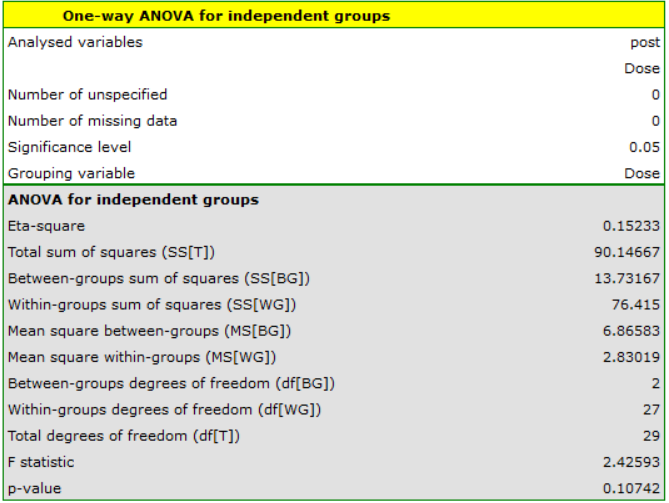
Unfortunately, the researcher did not get confirmation of the differences between the results.

Let's imagine that the researcher, realized that whether a drug would change cholesterol levels might be related to the patient's baseline cholesterol level and age. Therefore, he decided to perform a univariate ANCOVA (the factor is the dose of the drug) taking into account pre-treatment cholesterol levels and age as co-variables.

This time, the ANOCVA result indicated that there were significant differences between cholesterol levels after different doses of the drug (p=0.00003):

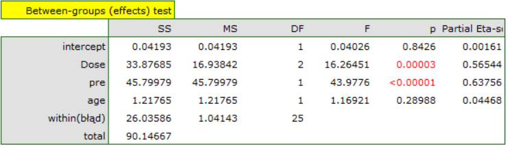
Including pre-test cholesterol levels reduced the obtained errors for the averages and narrowed the confidence intervals. To display the observed or expected averages, I choose the appropriate settings via Factor Options, to which I select the error graph. The first graph shows the observed averages with confidence interval, i.e., not including the effect of age and pre-treatment cholesterol levels; the second graph is the expected averages based on the built model with confidence intervals, i.e., after accounting for the effect of these two co-variables:

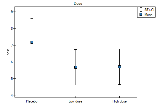
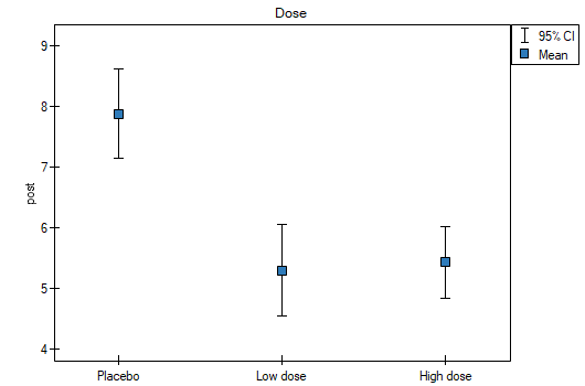
As a result, by taking into account the cholesterol level before treatment, the researcher was able to demonstrate the effectiveness of the new treatment. Cholesterol levels before treatment and age explain to some extent the changes in cholesterol levels after treatment, but we can attribute the rest of the changes in 57% to the drug dose used (partial Eta-square =0.565437). Post-hoc tests (selected by Factor options) suggested the formation of two homogeneous groups, the placebo group and the drug patient group, indicating that raising the dose to a high one does not make a difference, since the cholesterol levels obtained will be similar.

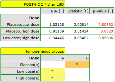
ANCOVA assumptions remained to be tested. Homogeneity of variance and constancy of slopes of simple regressions were confirmed using tests.

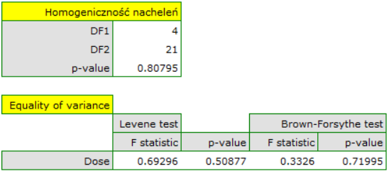
The normality of the rhesus distribution was assessed visually by plotting Q-Q plots:

Example (stress.pqs file)

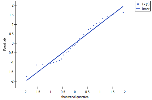
The example comes from the Datarium R-Cran package.

Researchers want to evaluate the effect of a new treatment and exercise on stress reduction after accounting for differences in age. The value of the stress measure is the interval outcome variable Y. Because the variables „treatment” and „exercise” have 2 and 3 categories, respectively, we will conduct a two-way ANCOVA to determine whether the interaction between exercise and treatment, while accounting for the subjects' age, is related to stress.

$\begin{tabular}{|c|c|} \hline \multicolumn{2}{|c|}{Factors}\\ treatment $X_1$ & exercise $X_2$ \\\hline \multirow{3}{*}{yes}& low \\\cline{2-2} & moderate \\\cline{2-2} & high\\\hline \multirow{3}{*}{no}& low \\\cline{2-2} & moderate \\\cline{2-2} & high\\\cline{2-2} \hline \end{tabular}$

In the analysis window, I set „stress” as the dependent variable, „treatment” and „exercise” as factors, and add the interaction of these two variables, the continuous co-variable is „age.”

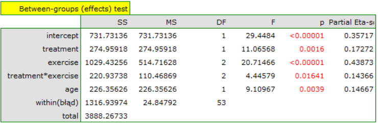
The result shows that the effect of treatment on stress varies with exercise intensity - indicated by a significant interaction of the two variables (p=0.016409). We plot a graph showing the expected mean stress levels for each of the six subgroups into which the interaction divided our data, and determine post-hoc tests.

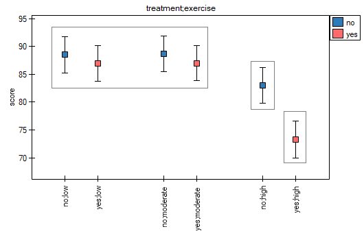
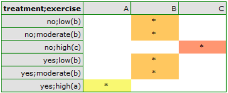
According to the results of the post-hoc test, we can speak of three different homogeneous groups: (B) the high-stress group is the group that exercises little or on average (whether or not they are treated sauropods), (C) the lower-stress group is the group that exercises a lot and is not treated, (A) the lowest-stress group is the group that exercises a lot and is treated. The values of the individual averages with confidence intervals are shown in the table

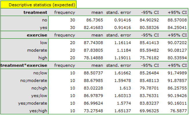
Assumptions regarding equality of variances, slopes of regression lines and normality of model residuals are met.

2023/03/31 19:17 · admin

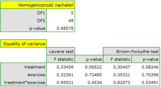
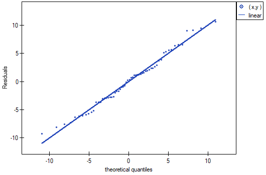
Mediation effect

Baron and Kenny (1986)⁸⁾ defined a mediator (M) as a variable that significantly explains the relationship between the independent variable (X) and the outcome variable (Y). In mediation, the relationship between the independent variable and the dependent variable is assumed to be an indirect effect that exists due to the influence of a third variable (mediator).

$\begin{pspicture}(-0.5,-0.5)(4,3.5) \psline{->}(0.2,3)(2.8,3) \rput(-2,3){\scriptsize one-dimensional model} \rput(0,2.8){\scriptsize \textbf{X}} \rput(3,2.8){\scriptsize \textbf{Y}} \rput(1.5,2.7){\scriptsize $\tau$} \rput(-2,0){\scriptsize multidimensional model} \rput(0,0){\scriptsize \textbf{X}} \rput(3,0){\scriptsize \textbf{Y}} \rput(1.5,2){\scriptsize \textbf{M}} \psline[linewidth=0.7pt, linestyle=dotted]{->}(0.2,0.2)(1.2,1.8) \psline[linewidth=0.7pt, linestyle=dotted]{->}(1.8,1.8)(2.8,0.2) \psline{->}(0.2,0)(2.8,0) \rput(0.4,1){\scriptsize \textit{a}} \rput(2.6,1){\scriptsize \textit{b}} \rput(1.5,-0.2){\scriptsize $\tau'$} \end{pspicture}$

We determine the magnitude of change by the difference in the coefficients describing the relationship between variable X and variable Y in the univariate model:

$Y=\tau\cdot X+c$

and in the multivariate model, that is, including the variable M:

$Y=\tau\cdot X+b\cdot M+c$ .

Difference:

$\begin{displaymath} \tau-\tau'=a\cdot b \end{displaymath}$

Mediation effect:

$\begin{displaymath} \frac{\tau-\tau'}{\tau}\cdot 100\% \end{displaymath}$

As a result, when the mediator (M) is included in the regression model that determines the relationship between the variable X and Y, the influence of the independent variable $\tau$ is reduced to $\tau'$ .

Tests to evaluate the mediation effect

The Sobel (1982)⁹⁾ test, the Aroian (1947)¹⁰⁾ test popularized by Baron and Kenny ¹¹⁾, and the Goodman (1960)¹²⁾ test are tests that determine whether the reduction in the effect of the independent variable on the outcome variable, when a mediator is included in the model, is a significant reduction and therefore whether the mediation effect is statistically significant.

Hypotheses:

$\begin{array}{cl} \mathcal{H}_0: & \tau = \tau'\\ \mathcal{H}_1: & \tau \ne \tau', \end{array}$

The test statistic for the Sobel test has the form:

$\begin{displaymath} Z=\frac{a\cdot b}{\sqrt{b^2\cdot SE^2_a+ a^2 \cdot SE^2_b}} \end{displaymath}$

The test statistic for the Aroian test has the form:

$\begin{displaymath} Z=\frac{a\cdot b}{\sqrt{b^2\cdot SE^2_a+ a^2 \cdot SE^2_b + SE^2_a\cdot SE^2_b}} \end{displaymath}$

The test statistic for the Goodman test has the form:

$\begin{displaymath} Z=\frac{a\cdot b}{\sqrt{b^2\cdot SE^2_a+ a^2 \cdot SE^2_b - SE^2_a\cdot SE^2_b}} \end{displaymath}$

These statistics have an asymptotically (for large sizes) normal distribution.

The p-value, designated on the basis of the test statistic, is compared with the significance level $\alpha$ :

$\begin{array}{ccl} $ if $ p \le \alpha & \Longrightarrow & $ reject $ \mathcal{H}_0 $ and accept $ \mathcal{H}_1, \\ $ if $ p > \alpha & \Longrightarrow & $ there is no reason to reject $ \mathcal{H}_0. \\ \end{array}$

Note

The Sobel test, as well as the Aroian and Goodman test, are very conservative tests and are intended only for large samples (greater than 100 items).

The mediation effect analysis window is invoked by Advanced Statistics→Multidivariate models→Mediation effect.

EXAMPLE

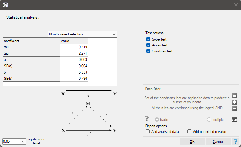
Based on the paper by Mimar Sinan Fine (2017) ¹³⁾.

The study includes 300 adults living in Istanbul. The dependent variable Y is systolic blood pressure and the independent variable X is age. The mediating variable M is the frequency of alcohol consumption. The purpose of this study is to investigate the relationship between age and systolic blood pressure and to present the effect of frequency of alcohol consumption on this relationship.

A one-dimensional model was built that did not account for the potential mediator:

$Y=0.319 \cdot X+c$ .

The effect size of variable X (age) on variable Y (systolic blood pressure) was tau=0.319.

A one-dimensional model was constructed that did not include a potential mediator:

The effect size of variable X (age) on variable Y (systolic blood pressure) was tau'=2.271. We also know from this model that b=5.333, and error $SE_b$ =0.786

The difference between the coefficients is tau-tau'= a*b=0.048. The effect of mediation is (tau-tau')/tau=(0.319-0.271)/0.371=0.15047, which means that M (frequency of alcohol consumption) modifies the relationship under study by decreasing the coefficient by about 15%.

A one-dimensional model was built to examine the effect of variable X on the mediator:

$M=0.009\cdot X+c$ .

We know from this model that the coefficient a=0.009, and the error $SE_a$ =0.004. We enter all this information in the analysis window obtaining the following report:

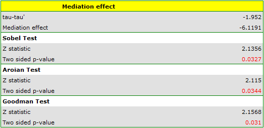
Based on the coefficients a and b and their standard errors, the result of Sobel (p=0.0327), Aroian (p=0.0344) and Goodman (p=0.0310) tests are determined. The obtained p-values indicate a statistically significant mediator. Thus, we confirmed that frequency of alcohol consumption affects the association of age with diastolic blood pressure so noticeably that it is worth explaining why this effect occurs.

2022/02/27 23:06 · admin

¹⁾

Rosenbaum P.R., Rubin D.B. (1983a), The central role of the propensity score in observational studies for causal effects. Biometrika; 70:41–55

²⁾

Austin P.C., (2009), The relative ability of different propensity score methods to balance measured covariates between treated and untreated subjects in observational studies. Med Decis Making; 29(6):661-77

³⁾

Austin P.C., (2011), An Introduction to Propensity Score Methods for Reducing the Effects of Confounding in Observational Studies. Multivariate Behavioral Research 46, 3: 399–424

⁴⁾

Normand S.L. T., Landrum M.B., Guadagnoli E., Ayanian J.Z., Ryan T.J., Cleary P.D., McNeil B.J. (2001), Validating recommendations for coronary angiography following an acute myocardial infarction in the elderly: A matched analysis using propensity scores. Journal of Clinical Epidemiology; 54:387–398.

⁵⁾

Green, S.B. (1991), How many subjects does it take to do a regression analysis? Multivariate Behavioral Research, 26, 499-510

⁶⁾

Savin N.E. and White K.J. (1977), The Durbin-Watson Test for Serial Correlation with Extreme Sample Sizes or Many Regressors. Econometrica 45, 1989-1996

⁷⁾

Peduzzi P., Concato J., Kemper E., Holford T.R., Feinstein A.R. (1996), A simulation study of the number of events per variable in logistic regression analysis. J Clin Epidemiol;49(12):1373-9

⁸⁾ , ¹¹⁾

Baron R. M., Kenny D. A. (1986), The moderator-mediator variable distinction in social psychological research: Conceptual, strategic and statistical considerations. Journal of Personality and Social Psychology, 51, 1173-1182.

⁹⁾

Sobel M. E. (1982). Asymptotic confidence intervals for indirect effects in structural equation models. Sociological Methodology 13: 290–312

¹⁰⁾

Aroian, L. A. (1947), The probability function of the product of two normally distributed variables. Annals of Mathematical Statistics, 18, 265-271.

¹²⁾

Goodman L. A. (1960), On the exact variance of products. Journal of the American Statistical Association, 55, 708-713

¹³⁾

Mimar S.F. (2017), The Mediation Analysis With the Sobel Test and the Percentile Bootstrap, International Journal of Management and Applied Science, Volume-3, Issue-2

PQStat - Baza Wiedzy

Pasek boczny

Spis treści

Multidimensional models

Preparation of variables for analysis

Matching groups

Interctions

Variables coding

Multiple Linear Regression

Model verification

More information about the variables in the model

Analysis of model residuals

Example for multiple regression

Model-based prediction and test set validation

Comparison of multiple linear regression models

Logistic regression

The Odds Ratio

Model verification

Graphs in logistic regression

Examples for logistic regression

Model-based prediction and test set validation

Comparison of logistic regression models

Factorial ANOVA - GLM

ANCOVA

Mediation effect

PQStat - Baza Wiedzy

Narzędzia użytkownika

Narzędzia witryny

Pasek boczny

Spis treści

Multidimensional models

Preparation of variables for analysis

Matching groups

Interctions

Variables coding

Multiple Linear Regression

Model verification

More information about the variables in the model

Analysis of model residuals

Example for multiple regression

Model-based prediction and test set validation

Comparison of multiple linear regression models

Logistic regression

The Odds Ratio

Model verification

Graphs in logistic regression

Examples for logistic regression

Model-based prediction and test set validation

Comparison of logistic regression models

Factorial ANOVA - GLM

ANCOVA

Mediation effect

Narzędzia strony