Spis treści

Randomness of point distribution
- Nearest Neighbor Analysis

Randomness of point distribution

To conduct analysis of the randomness of point distribution on the basis of a Map data we should have at our disposal a point, multipoint, or polygonal file. In the case of an analysis of a polygonal file, calculations are based on centroids of polygons, and in the case of a multipoint file they are based on centers of objects.

The effect of uniform dispersion appears when points are distributed more regularly than the possible result of random distribution. If the spatial distribution is as probable as any other distribution we speak about spatial randomness. When the points come in groups we speak about clustered distribution.

$\begin{pspicture}(1,-1)(12.5,4.5) \psline{-}(5,0)(5,4) \psline{-}(5,0)(9,0) \psline{-}(5,4)(9,4) \psline{-}(9,0)(9,4) \rput(7.12,1.31){$\circ$} \rput(5.63,3.33){$\circ$} \rput(6.56,3.86){$\circ$} \rput(8.18,0.04){$\circ$} \rput(5.08,0.91){$\circ$} \rput(8.4,2.98){$\circ$} \rput(5.03,3.61){$\circ$} \rput(7.46,3.33){$\circ$} \rput(6.7,1.23){$\circ$} \rput(8.43,3.06){$\circ$} \rput(7.66,3.75){$\circ$} \rput(5.82,1.7){$\circ$} \rput(5.01,2.85){$\circ$} \rput(7.4,0.67){$\circ$} \rput(6.68,2.48){$\circ$} \rput(7.42,2.03){$\circ$} \rput(8.3,0.93){$\circ$} \rput(8.82,2.14){$\circ$} \rput(6.62,3.86){$\circ$} \rput(6.73,1.99){$\circ$} \rput(5.9,2.11){$\circ$} \rput(7.73,1.51){$\circ$} \rput(7.53,0.08){$\circ$} \rput(5.72,1.52){$\circ$} \rput(8.92,3.77){$\circ$} \psline{-}(0,0)(0,4) \psline{-}(0,0)(4,0) \psline{-}(0,4)(4,4) \psline{-}(4,0)(4,4) \rput(0,0){$\circ$} \rput(0,1){$\circ$} \rput(0,2){$\circ$} \rput(0,3){$\circ$} \rput(0,4){$\circ$} \rput(1,0){$\circ$} \rput(1,1){$\circ$} \rput(1,2){$\circ$} \rput(1,3){$\circ$} \rput(1,4){$\circ$} \rput(2,0){$\circ$} \rput(2,1){$\circ$} \rput(2,2){$\circ$} \rput(2,3){$\circ$} \rput(2,4){$\circ$} \rput(3,0){$\circ$} \rput(3,1){$\circ$} \rput(3,2){$\circ$} \rput(3,3){$\circ$} \rput(3,4){$\circ$} \rput(4,0){$\circ$} \rput(4,1){$\circ$} \rput(4,2){$\circ$} \rput(4,3){$\circ$} \rput(4,4){$\circ$} \psline{-}(10,0)(10,4) \psline{-}(10,0)(14,0) \psline{-}(10,4)(14,4) \psline{-}(14,0)(14,4) \rput(10.79,0.61){$\circ$} \rput(11.21,0.84){$\circ$} \rput(11.32,1.11){$\circ$} \rput(11.37,0.58){$\circ$} \rput(10.7,0.34){$\circ$} \rput(10.43,0.58){$\circ$} \rput(10.58,0.17){$\circ$} \rput(10.62,0.41){$\circ$} \rput(11.61,0.31){$\circ$} \rput(10.47,0.84){$\circ$} \rput(12.93,3.06){$\circ$} \rput(13.23,3.69){$\circ$} \rput(12.59,2.84){$\circ$} \rput(13.42,3.27){$\circ$} \rput(13.67,2.91){$\circ$} \rput(13.08,2.94){$\circ$} \rput(13.4,3.33){$\circ$} \rput(13.3,3.68){$\circ$} \rput(12.66,3.3){$\circ$} \rput(10.98,3.66){$\circ$} \rput(11.31,3.45){$\circ$} \rput(11.43,3.36){$\circ$} \rput(13.54,0.4){$\circ$} \rput(13.86,0.38){$\circ$} \rput(13.31,0.53){$\circ$} \psline[linewidth=3pt]{<->}(0,-0.5)(14,-0.5) \rput(1.5,-1){uniform distribution} \rput(7,-1){random distribution} \rput(13,-1){clustered distribution} \end{pspicture}$

Nearest Neighbor Analysis

In the Nearest Neighbor Analysis the boundaries of the area in which the analysed points are enclosed have the crucial influence on the result. The example below illustrates regularly distributed points and their clustered distribution when bounded by a large rectangle.

$\begin{pspicture}(1,0)(12.5,3) \psline[linestyle=dashed](5,0)(5,2.5) \psline[linestyle=dashed](5,0)(8,0) \psline[linestyle=dashed](5,2.5)(8,2.5) \psline[linestyle=dashed](8,0)(8,2.5) \psline{-}(5.7,0.5)(5.7,2) \psline{-}(5.7,0.5)(7.3,0.5) \psline{-}(5.7,2)(7.3,2) \psline{-}(7.3,0.5)(7.3,2) \rput(6.2,1){$\circ$} \rput(6.8,1.5){$\circ$} \rput(6.2,1.5){$\circ$} \rput(6.8,1){$\circ$} \end{pspicture}$

Depending on the needs, the bounding can be defined with the help of: a convex hull, the smallest rectangle, a rectangle from layer bounding, or the smallest circle. The studied area can also be defined only with the use of the size of its area.

The distance between the points is measured with the Euclidean metric.

The first stage of the nearest neighbor analysis is calculating the distance among all points. Next, for each point we search for the nearest point, i.e. for the nearest neighbor ( $NN$ ).

Note

The distances between all points are defined by a spatial weight matrix. In Moran's analysis window we can choose matrix generated previously by using menu Spatial analysis → Tools → Spatial weights matrix or indicate the neighbor matrix according to contiguity – Queen, row standardized, that is proposed by the program.

The basic statistics for the analysis of the nearest neighbors are:

$d_i(NN)$ – the distance of each point from its nearest neighbor,
$\overline{NN}$ – the mean nearest neighbor distance:

$\begin{displaymath} \overline{NN}=\sum_{i=1}^n\frac{d_i(NN)}{n} \end{displaymath}$

$SD_{(NN)}$ – standard deviation of the nearest neighbors distance,
$\overline{ran}$ – mean random nearest neighbor distance:

$\begin{displaymath} \overline{ran}=\frac{0.5}{\sqrt{\frac{n}{A}}} \end{displaymath}$

Nearest Neighbor Index

Nearest Neighbor Index ( NNI) is based on a method described by botanists: Clark and Evans (1954) ¹⁾. $NNI$ compares distances observed between the nearest points, and distances which would appear for a random distribution of points.

$\begin{displaymath} NNI=\frac{\overline{NN}}{\overline{ran}} \end{displaymath}$

When the compared distances are the same then $NNI=1$ . When the observed distances between the nearest points are smaller than expected then the points are nearer to one another than in a random distribution, and $NNI<1$ . In such a case, clusters occur. When the situation is reverse, then $NNI>1$ , which points to the occurrence of the effect of uniform distribution, i.e. points are distributed more regularly than in a case of random distribution.

Significance of the Nearest Neighbor Index

The test for checking the significance of the Nearest Neighbor Index $NNI$ serves the purpose of verifying the hypothesis that the distances observed between the nearest points are the same as the expected distances which would appear in a random distribution of points.

Hypotheses:

$\begin{array}{cl} \mathcal{H}_0: & NNI = 1, \\ \mathcal{H}_1: & NNI \ne 1. \end{array}$

The test statistic has the form presented below:

$\begin{displaymath} Z=\frac{\overline{NN}-\overline{ran}}{SE_{\overline{ran}}}, \end{displaymath}$

where:

$\begin{array}{cl} SE_{(ran)} = \sqrt{\frac{4-\pi A}{4\pi n^2}} & \textrm{-- standard error of the mean random}\\ &\textrm{nearest neighbor distance } \end{array}$

Statistics $Z$ asymptotically (for a large sample size) has the normal distribution.

The p-value, designated on the basis of the test statistic, is compared with the significance level $\alpha$ :

$\begin{array}{ccl} $ if $ p \le \alpha & \Longrightarrow & $ reject $ \mathcal{H}_0 $ and accept $ \mathcal{H}_1, \\ $ if $ p > \alpha & \Longrightarrow & $ there is no reason to reject $ \mathcal{H}_0. \\ \end{array}$

Analysis of Subsequent Nearest Neighbors

To analyse subsequent nearest neighbors one takes into account the distance to the second nearest neighbor, the third nearest neighbor, and so on, to the $k$ -order nearest neighbor. For the neighborhood of each order (from the nearest neighbor to the $k$ -order neighbor) subsequent Nearest Neighbor Indexes $k_{ordered}NNI$ are calculated:

$\begin{displaymath} k_{ordered}NNI=\frac{k_{ordered}\overline{NN}}{k_{ordered}\overline{ran}} \end{displaymath}$

where:

$\displaystyle k_{ordered}\overline{NN}$ – mean distance from neighbors of $k$ -order,

$\displaystyle k_{ordered}\overline{ran}=\frac{k(2k)!}{\left(2^kk!\right)^2\sqrt{\frac{n}{A}}}$ – mean random distance from neighbors of $k$ -order.

The results of the point density analysis conducted for subsequent neighbors can be presented on a graph so as to illustrate the placement of $NNI$ in reference to the line which shows the random point structure and so as to check if a growing or falling trend has been achieved for the indexes.

Edge Effect

Objects placed near the bounding show a tendency to be further away from their nearest neighbors than other objects within the analysed area. The reason for it is the simple fact that the nearest neighbors of the objects near the border can be objects outside the studied area. In such a situation we can conduct an analysis with an adjustment for the edge effect. In such a case the distance of a point from its nearest neighbor ( $d_i(NN)$ ) is calculated as the minimum distance of the point from its neighbors and from the boundary. Thus, if the distance of the point from the boundary will be smaller than the distance from its neighbors, then the distance from the boundary is considered to be $d_i(NN)$ . However, such a calculation of the nearest neighbor requires an assumption that there will always be a neighboring point on the border.

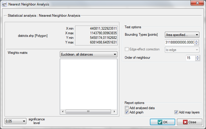
The window with settings for Nearest Neighbor Analysis is accessed via the menu Spacial analysis → Spatial Statistics → Nearest Neighbor Analysis.

EXAMPLE (directory: districts, SHP files: districts)

The admistrative division of Poland into powiats should, by definition, be uniform. With the use of NNI we will check if that is the case.

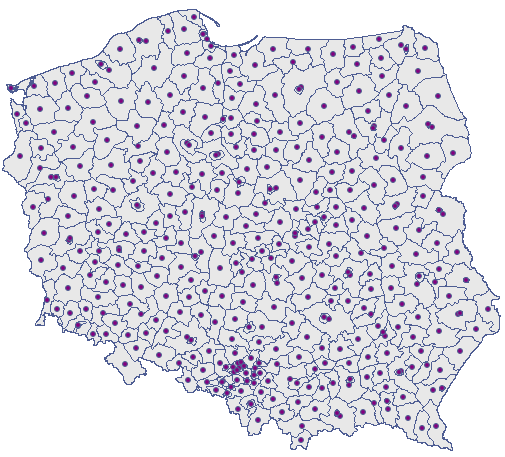
The districts map contains information about locations of polygons (Polish powiats).

The nearest neighbor analysis will be based on centroids representing powiats. We can draw them (add the centroid layer to the map of powiats) with the use of the Map manager.

The nearest neighbor analysis will be made with the use of information about the size of the area of Poland – it is $311888000000m^2$ . Apart from the nearest neighbor index we will also calculate the indices of subsequent neighbors, up to 15.

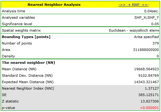
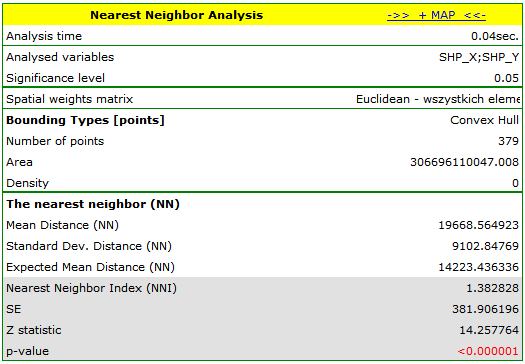
After entering the size of the area in the analysis window, a nearest neighbor index amounting to 1.37127 was received. Its statistical significance was ( $p<0.000001$ ), greater than value 1. The mean distance between the nearest neighboring centroids is $19668.564923m$ and the standard deviation is $9102.84769m$ . We will receive a very similar result when we return to the analysis (the button ) and choose the convex hull as the bounding ( $NNI=1.382828$ , $p<0.000001$ ).

We add the boundaries defined by the convex hull by pressing the button 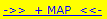and choosing the layer of bounding.

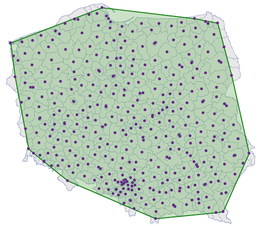
The correction of the effect of a boudary defined in this way lowers the value of $NNI$ to 1.340503 but leaves the general tendency of the subsequent nearest neighbor indices unchanged.

In each of the analysis described above the subsequent neighbor indices are greater than 1 and, although they initially approximate 1, from order 5 they stabilize at the level of about 1.1. The result, then, confirms the uniform distribution of Polish powiats.

EXAMPLE (directory: poplar, SHP files: T-poplar, S-poplar)

Competition among species has an influence on the changes in the distribution of particular species of plants and on their density. Competition within a species is usually stronger than that among different species as members of the same species have almost identical demands and compete for the same resources. The intensity of competition within a species increases with the growth of the population. To check the influence of the competition on a certain species of balsamic poplar, a wooded area not regulated by man was studied. Locations of young trees and of old ones were studied.

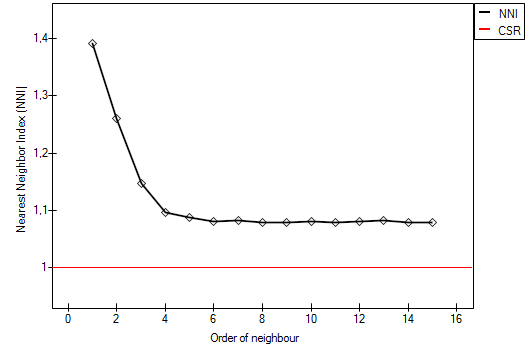
Mapa T-poplar contains fictitious information about the locations of 121 points (old balsamic poplars) in a rectangular wooded area.
Mapa S-poplar contains fictitious information about the locations of 326 points (young balsamic poplars) in a rectangular wooded area.

On the map young poplars were marked in red and old poplars were marked in blue.

On the basis of the nearest neighbor indices, the structure of poplar density was compared in the area defined by a rectangle of layer bounding.

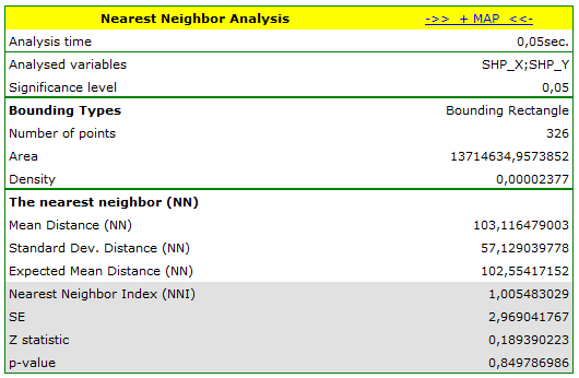
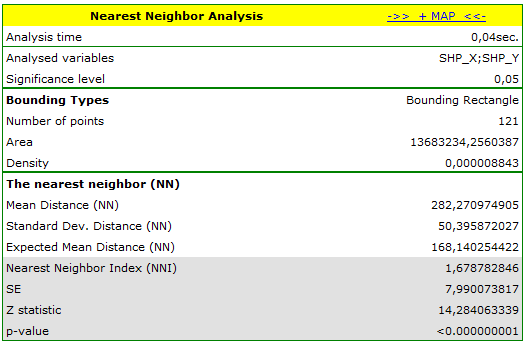
Young poplars have greater density than old ones. Their mean nearest neighbor distance is $103.12m$ whereas for old poplars the value is $282.27m$ . Due to competition in the development of the structure of forest stand the spatial pattern for old trees is more regular ( $NNI=1.68$ , $p<0.000001$ ) than the one for young poplars ( $NNI=1.01$ , $p=0.8498$ ).