PQStat - Baza Wiedzy

Spis treści

Spatial analysis - an introduction

Spatial analysis - an introduction

Basic definitions

Geographic Information System - GIS – is a system for entering, storing, processing, and visualization of geographic data. From the technical point of view GIS is a tool which allows the analysis of interrelated:

information about spatial locations of objects – represented by means of a map;
descriptive characteristic concerning objects presented on a map – represented by means of a database.

Objects represented by means of a map are:

Points – the location of which, in 2D, is defined with the help of two coordinates $(x,y)$ ;
Multipoints – they are points grouped in sets:

$\begin{pspicture}(3,0)(3,2.5) \rput(0.5,1){$\bullet$} \rput(1,2.3){$\circ$} \rput(0.5,1.7){$\bullet$} \rput(2.7,1.55){$\circ$} \rput(3,1.1){$\star$} \rput(0.7,0.3){$\circ$} \rput(1.2,1.2){$\bullet$} \rput(2.05,2.2){$\circ$} \rput(1.6,2.2){$\circ$} \rput(2.4,1.7){$\star$} \rput(2.9,0.6){$\star$} \rput(-1,2){$1)$} \end{pspicture}$ An example of a multipoint in which each point is defined as belonging to one of 3 groups.

Lines – they are created by linking subsequent points, in proper order (lines can intersect);
Polygons – they are closed spaces, restricted by means of external rings (closed lines which do not intersect and which go through at least 3 points, in an appropriate order). Polygons can also contain internal rings constituting their internal boundaries. External rings are defined clockwise and the internal ones the other way round.

$\begin{pspicture}(-1,-1)(12,6) \psline{<-}(1,4)(0,0) \psline{<-}(3,5)(1,4) \psline{<-}(4,2)(3,5) \psline{<-}(3,1)(4,2) \psline{<-}(0,0)(3,1) \rput(1.9,-.7){$1)$} \psline{<-}(8,4)(7,0) \psline{<-}(10,5)(8,4) \psline{<-}(11,2)(10,5) \psline{<-}(10,1)(11,2) \psline{<-}(7,0)(10,1) \psline{->}(9.4,3)(10,2) \psline{->}(10,2)(10.5,2.8) \psline{->}(10.5,2.8)(9.3,3.5) \psline{->}(9.3,3.5)(9.4,3) \psline{->}(8.4,2)(8.8,1) \psline{->}(8.8,1)(9.3,1.3) \psline{->}(9.3,1.3)(8.3,2.7) \psline{->}(8.3,2.7)(8.4,2) \rput(8.9,-.7){$2)$} \end{pspicture}$

1) An example of a polygon which only has an external boundary (with no internal rings);
2) An example of a polygon which has both an external boundary and internal boundaries (areas defined by the internal rings constitute a part of an external area, i.e. they do not belong to the polygon).

Object attributes are entered into the base in the form of:

numbers – e.g. area, temperature,

texts – e.g. names of objects.

Map projection is a mathematical method of mapping the surface of the Earth onto a map surface. There is a number of methods for such mapping. The mappings can be based on a spheroid or on the surface of a ball (a sphere), or on a part of either of them. Each mapping forms the basis for defining an appropriate coordinate system. Because each projection of a surface entails certain distortions (distortions of angles, areas, lengths), the choice of a proper system depends on the aim for which the map is to be used.

Coordinate systems used in cartography are classified as:

geographic coordinate systems (they define geographic latitude and longitude);
cartesian coordinate systems;
polar coordinate systems.

For a map to be loaded correctly, the program PQStat requires a vector map saved in a SHAPEFILE (shp) type of file and defined in a proper Cartesian coordinate system, with line scale.

The program tries to automatically detect maps with geographic coordinates. If, while importing the map, the program detects a geographic coordinate system, it suggests converting the coordinates into a UTM system (Universal Transverse Mercator), on the basis of the WGS-84 system of reference. As conversion might be incorrect (due to the use of many geographic coordinate system and the lack of certainty with regard to the applied system), it is recommended that properly prepared maps be used – in a Cartesian coordinate system.

2022/02/09 12:56

Map opening

A map with the attribute file assigned to the map can be loaded via:

import of a shapefile, SHP, into the datasheet,
loading the PQS/PQX file which contains data from shapefiles (SHP).

Import of a Shapefile (SHP)

Import is made by choosing the menu option File→Import data…→SHP/SHX/DBF ESRI Shapefile (*.shp).

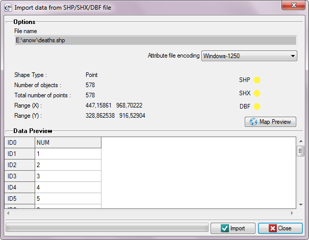
In the import window we can preview the imported map and its attributes saved in a DBF file. If the directory from which we import contains all files necessary for loading the map then the correct reading of appropriate files is confirmed in yellow by proper controls. Attributes ascribed to a shapefile, in the form of a DBF database, are not required for proper loading of a map. An attribute table can be completed after a map file has been loaded, by filling in proper cells of the datasheet linked with the map.

2022/02/09 12:56

How to reduce a workspace

Workspace is limited for the purpose of indicating only those objects which will be subjected to the analysis. Such objects are indicated in the program by activating or deactivating them. Inactive objects are not subjected to statistical analyses.

Manual activation/deactivation of objects

Indicating a row in the data sheet which describes the appropriate object and selecting the option Activate/Deactivate from the context menu on its name;
Indicating an object on the map and selecting, from the context menu, the option Activate/Deactivate or Identify → Activate/Deactivate object.
Automatic activation/deactivation of objects

Selecting objects on the basis of data sheet – for example, one can indicate as active only those shops which are groceries with an area not larger than 1000m2. In such a case, the setting of appropriate conditions for selecting objects takes place in the window of Activation/Deactivation available after selecting the Edit →Activate/Deactivate (filter)… menu. A detailed description of the manners of selection of that type can be found in the User Manual - PQStat (Chapter: How to Reduce Data Sheet Workspace).
Selecting objects on the basis of a map – for example, one could only distinguish those shops which are within a rectangular or elliptical area marked on a map. We select the area with the use of the selection area tools (selection area tools) and later activate or deactivate in the window Activate/Deactivate in the selection available after selecting the Tools →Activate/Deactivate in the selection menu in the window of the Map manager.

In order to activate all objects one should select the Tools →Activate all menu in the window of the Map manager or the Edit →Activate all menu in the window of PQStat.

2022/02/09 12:56

Geometric calculations

Geometric calculations are formulas (read the User Manual - PQStat (Chapter: Formulas)). The formulas can pertain data which describe map geometry and data visible in a datasheet.

Formulas for data which describe map geometry - geometric/geographic functions

Data for transformation are chosen from a shapefile (SHP)

Available formulas:

meanCenter (poly) - gives center coordinates for polygons,

centroid (poly) - gives centroid coordinates for polygons,

area (poly) - gives polygon areas,

perimeter (poly) - gives polygon perimeters.

Formulas for data visible in a datasheet - creating maps

Available formulas:

map (points) - gives a vector map presenting points together with assigned datasheet.

2022/02/09 12:56

Testing hypotheses

Verification of statistical hypotheses is checking certain assumptions formulated for parameters of a general population on the basis of results from a sample.

Formulation of hypotheses which will be verified with the help of statistical tests.

Each statistical test gives the general form of a null hypothesis – $\mathcal{H}_0$ and of an alternative hypothesis – $\mathcal{H}_1$ :

$\begin{array}{cl} \mathcal{H}_0: & \textrm{\textbf{in the studied population} \textcolor{red}{\textbf{THERE IS NOT}} a statistically significant}\\ &\textrm{\quad e.g. dependence},\\ &\textrm{\quad e.g. difference},\\ &\textrm{\quad ...}\\ &\textrm{\textbf{between}}\\ &\textrm{\quad e.g. spatial distribution},\\ &\textrm{\quad e.g. presence of particular values},\\ &\textrm{\quad ...}\\ &\textrm{\textbf{in the analysed area}},\\\\ \mathcal{H}_1: & \textrm{\textbf{in the studied population} \textcolor{red}{\textbf{THERE IS}} a statistically significant}\\ &\textrm{\quad e.g. dependence},\\ &\textrm{\quad e.g. difference},\\ &\textrm{\quad ...}\\ &\textrm{\textbf{between}}\\ &\textrm{\quad e.g. spatial distribution},\\ &\textrm{\quad e.g. presence of particular values},\\ &\textrm{\quad ...}\\ &\textrm{\textbf{in the analysed area}}.\\\\ \end{array}$

Example:

$\begin{array}{cl} \mathcal{H}_0: & \textrm{THERE IS NOT a statistically significant dependence between the spatial distribution}\\ &\textrm{of chemist's shops in Wielkopolska -- we assume that their distribution in }\\ &\textrm{the studied area is random}.\\ \end{array}$

If we do not know if the distribution of the shops can be more regular than random distribution, or the other way round – more clustered than random distribution, then the alternative hypothesis should be two-sided, i.e. we do not presume a particular direction:

$\begin{array}{cl} \mathcal{H}_1: & \textrm{THERE IS a statistically significant dependence between the spatial distribution}\\ &\textrm{of chemist's shops in Wielkopolska -- we assume that their distribution in }\\ &\textrm{the given area is not random, i.e. we presume the presence of 2 directions: a distribution}\\ &\textrm{which is more regular than random distribution and a distribution which is more clustered than}\\ &\textrm{random distribution}.\\ \end{array}$

It may happen (in very rare cases) that we are certain that we know the direction in the alternative hypothesis. We can then utilize a one-sided alternative hypothesis.

Hypothesis Verification

To check which of the hypotheses, $\mathcal{H}_0$ or $\mathcal{H}_1$ , is more probable, we select a proper statistical test.

Test statistic of a chosen test, calculated according to its formula, is subjected to the theoretical distribution appropriate for that statistic.

$\psset{xunit=1.25cm,yunit=10cm} \begin{pspicture}(-5,-0.1)(5,.5) \psline{->}(-4,0)(4.5,0) \psTDist[linecolor=green,nue=4]{-4}{4} \pscustom[fillstyle=solid,fillcolor=cyan!30]{% \psTDist[linewidth=1pt,nue=4]{-4}{-2.776445}% \psline(-2.776445,0)(-4,0)} \pscustom[fillstyle=solid,fillcolor=cyan!30]{% \psline(2.776445,0)(2.776445,0)% \psTDist[linewidth=1pt,nue=4]{2.776445}{4}% \psline(4,0)(2.776445,0)} \rput(-3.6,0.2){$\alpha/2$} \psline{->}(-3.6,0.15)(-3.1,0.04) \rput(3.6,0.2){$\alpha/2$} \psline{->}(3.6,0.15)(3,0.04) \rput(1,0.5){$1-\alpha$} \psline{->}(1,0.46)(0.55,0.35) \rput(2.5,-0.04){value of test statistic} \end{pspicture}$

The program calculates the value of a test statistic and $p$ -value for that statistic (that is the part of the area under the curve which corresponds to the value of the test statistic). Value $p$ allows to choose which hypothesis, the null hypothesis or the alternative hypothesis, is more probable. The truth of the null hypothesis is always presumed and the proofs gathered in the data are to provide a sufficient number of arguments against that hypothesis:

$\begin{array}{ccl} $ if $ p \le \alpha & \Longrightarrow & $ reject $ \mathcal{H}_0 $ and accept $ \mathcal{H}_1, \\ $ if $ p > \alpha & \Longrightarrow & $ there is no reason to reject $ \mathcal{H}_0. \\ \end{array}$

Usually, significance level $\alpha=0.05$ is chosen with the acceptance of the premise that in 5\% of situations the null hypothesis will be rejected being a true one. In special cases a different significance level, e.g. 0.01 or 0.001, can be set.

2022/02/09 12:56

PQStat - Baza Wiedzy

Narzędzia użytkownika

Narzędzia witryny

Pasek boczny

Spis treści

Spatial analysis - an introduction

Basic definitions

Map opening

How to reduce a workspace

Geometric calculations

Testing hypotheses

Narzędzia strony