PQStat - Baza Wiedzy

Similarity matrix

The relationship between objects can be expressed by their distances or more generally by their dissimilarity. The further apart the objects are, the more dissimilar they are, while the closer together they are, the greater their similarity. It is possible to examine the distance of objects in terms of many features, e.g. when compared objects are cities, their similarity can be defined, among others, based on: length of the road that connects them, population density, GDP per capita, pollution emissions, average real estate prices, etc. With so many different features you have to choose the measure of distance in such a way, that it best reflects the actual similarity of objects.

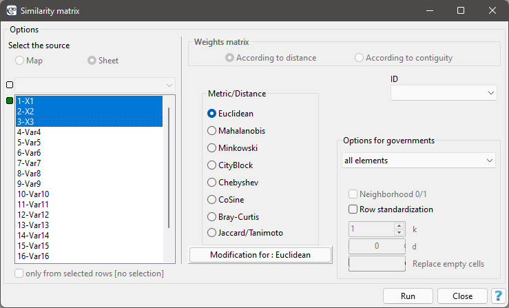
The window with the settings for the macierzy podobieństwa options is opened via Data→Matrices…

We express the dissimilarity/similarity of objects by means of distances which are most often metrics. However, not every measure of distance is a metric. For a distance to be called a metric it must meet 4 conditions:

the distance between objects cannot be negative: $d(x_1, x_2) \geq 0$ ,
the distance between two objects is 0 if and only if they are identical: $d(x_1, x_2) = 0 \Longleftrightarrow x_1 = x_2$ ,
the distance must be symmetric, i.e., the distance from object $x_1$ to $x_2$ must be the same as from $x_2$ to $x_1$ : $d(x, y) = d(y, x)$ ,
the distance must meet the triangle requirement: $d(x, z) \leq (x, y) + d(y, z)$ .

Note

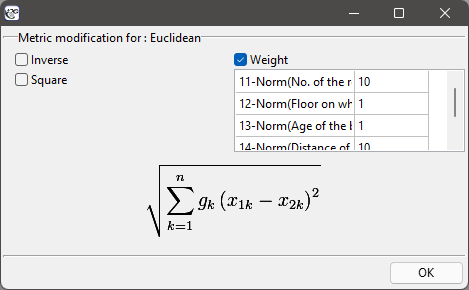
Metrics should be calculated for features with the same value ranges. If not, then features with higher ranges would have a greater impact on the similarity score than those with lower ranges. For example, when calculating similarity between people, we can base it on such features as body mass and age. Then body mass in kilograms, in the range of 40 to 150 kg, will have a greater influence on the result than age in years, in the range of 18 to 90 years. To ensure that the effect of each characteristic on the resulting similarity score is balanced, you should normalize/standarize each characteristic before proceeding with the analysis. On the other hand, if you want to decide the magnitude of this influence yourself, after applying the standardization, indicating the type of metric, you should enter the weights you gave yourself.

Distance/Metrics:

Euclidean

When talking about distance without defining its type, one assumes that it is Euclidean distance - the most common type of distance that is a natural part of real world models. Euclidean distance is a metric and is given by the formula:

$\begin{displaymath} d(x_1,x_2)=\sqrt{\sum_{k=1}^n\left(x_{1k}-x_{2k}\right)^2} \end{displaymath}$

Minkowski

The Minkowski distance is defined for parameters $p$ and $r$ equal to each other - it is then a metric. This type of metric allows one to control the similarity calculation process by specifying values of $p$ and $r$ included in the formula:

$\begin{displaymath} d(x_1,x_2)=\sqrt[p]{\sum_{k=1}^n\left|x_{1k}-x_{2k}\right|^r} \end{displaymath}$

Increasing the parameter $r$ increases the weight assigned to the difference between objects for each feature, changing $p$ gives more/less importance to closer/farther objects. If $r$ and $p$ are equal to 2, Minkowski distance reduces to Euclidean distance, if they are equal to 1, to CityBlock distance, and with these parameters approaching infinity, to Chebyshev metric.

CityBlock (otherwise: Manhattan distance or cab distance)

This is a distance that allows you to move in only two directions perpendicular to each other. This type of distance is similar to moving on perpendicularly intersecting streets (a square street grid that resembles the layout of Manhattan). This metric is given by the formula:

$\begin{displaymath} d(x_1,x_2)=\sum_{k=1}^n|x_{1k}-x_{2k}| \end{displaymath}$

Chebyshev

The distance between the objects being compared is the greatest of the distances obtained for each characteristic of those objects:

$\begin{displaymath} d(x_1,x_2)=\max_{k}|x_{1k}-x_{2k}| \end{displaymath}$

Mahalanobis

Mahalanobis distance is also called statistical distance. It is a distance weighted by the covariance matrix, by which objects described by mutually correlated characteristics can be compared. The use of Mahalanobis distance has two main advantagesi:

1) Variables for which larger variances or larger ranges of values are observed do not have an increased effect on the Mahalanobis distance score (since when using a covariance matrix you standardize the variables using the variance located on the diagonal). As a result, there is no requirement to standardize/normalize the variables before proceeding with the analysis.

2) It takes into account the mutual correlation of the characteristics describing the compared objects (using the covariance matrix it uses the information about the relationship between the characteristics located outside the diagonal of the matrix).

$\begin{displaymath} d(x_1,x_2)=\sqrt{(\vec{x}-\vec{y})^TS^{-1}(\vec{x}-\vec{y})} \end{displaymath}$ The measure calculated in this way meets the conditions of the metric.

CoSine

The Cosine distance should be calculated using positive data because it is not a metric (it does not meet the first condition: $d(x_1, x_2) \geq 0$ ). So if you have features that also take negative values you should transform them beforehand using, for example, normalization to an interval spanned by positive numbers. The advantage of this distance is that (for positive arguments) it is limited to the range [0, 1]. The similarity of two objects is represented by the angle between two vectors representing the features of those objects.

$\begin{displaymath} d(x_1,x_2)=1-K, \end{displaymath}$

where $K$ is the similarity coefficient (cosine of the angle between two normalized vectors):

$\begin{displaymath} K=\frac{\sum_{k=1}^nx_{1k}x_{2k}}{\sqrt{\sum_{k=1}^nx_{1k}^2}\sqrt{\sum_{k=1}^nx_{2k}^2}} \end{displaymath}$

Objects are similar when the vectors overlap - then the cosine of the angle (similarity) is 1 and the distance (dissimilarity) is 0. Objects are different when the vectors are perpendicular - then the cosine of the angle (similarity) is 0 and the distance (dissimilarity) is 1.

Example - comparing texts

Text 1: several people got on at this stop and one person got off at the next stop

Text 2: at the bus stop, one lady got off and several got on

One wants to know how similar the texts are in terms of the number of the same words, but is not interested in the order in which the words occur.

You create a list of words from both texts and count how often each word occurred:

$\begin{tabular}{|c||c|c|c|c|c|c|c|c|c|c|c|c|} \hline \textbf{tekst 1}&2&1&1&1&1&1&1&1&1&1&0\\ \textbf{tekst 2}&1&0&1&1&1&0&1&0&1&1&1\\\hline \end{tabular}$

The cosine of the angle between the vectors is 0.784465, so the distance between them is not large $d(tekst_1,tekst_2)=1-0,784465=0.215535$ .

In a similar way, you can compare documents by the occurrence of keywords to find those most relevant to the search term.

Bray-Curtis

The Bray-Curtis distance (measure of dissimilarity) should be calculated using positive data because it is not a metric (it does not meet the first condition: $d(x_1, x_2) \geq 0$ ). If you have features that also take negative values, you should transform them beforehand using, for example, normalization to an interval spanned by positive numbers. The advantage of this distance is that (for positive arguments) it is limited to the interval [0, 1], where 0 - means that the compared objects are similar, 1 - dissimilar.

$\begin{equation} d(x_1,x_2)=\frac{\sum_{k=1}^n|x_{1k}-x_{2k}|}{\sum_{k=1}^n(x_{1k}+x_{2k})} \end{equation}$

In calculating the similarity measure $BC$ , we subtract the Bray-Curtis distance from the value 1:

$\begin{equation} BC=1-d(x_1,x_2) \end{equation}$

Jaccard

Jaccard's distance (measure of dissimilarity) is calculated for binary variables (Jaccard, 1901), where 1 indicates the presence of a feature 0- its absence.

$\begin{tabular}{|c|c||c|c|} \hline \multicolumn{2}{|c||}{ }& \multicolumn{2}{|c|}{object 1}\\\cline{3-4} \multicolumn{2}{|c||}{ }& 1 & 0 \\\hline \hline \multirow{2}{*}{object 2}& 1 & a & b \\\cline{2-4} & 0 & c & d\\\hline \end{tabular}$

The Jacckard distance is expressed by the formula:

$\begin{equation} d(x_1,x_2)=1-J. \end{equation}$

where:

$J=\frac{a}{a+b+c}$ - Jaccard similarity coefficient.

Jaccard similarity coefficient is in the range [0,1], where 1 means the highest similarity, 0 - the lowest. Distance (dissimilarity) is interpreted in the opposite way: 1 - means that the compared objects are dissimilar, 0 - that they are very similar. The meaning of Jaccard's similarity coefficient is well described by the situation involving the choice of goods by customers. By 1 we denote the fact that the customer bought the given product, 0 - the customer did not buy this product. Calculating the Jaccard coefficient you compare 2 products to find out what part of the customers buy them in together. Of course we are not interested in information about customers who did not buy either of the compared items. Instead, we are interested in how many people who choose one of the compared products choose the other one at the same time. The sum $a+b+c$ - is the number of customers who chose either of the compared items, $a$ - is the number of customers choosing both items at the same time. The higher Jaccard's similarity coefficient, the more inseparable the products are (the purchase of one is accompanied by the purchase of the other). The opposite will happen when we get a high Jaccard dissimilarity coefficient. It will indicate that the products are highly competitive, i.e. the purchase of one will result in the lack of purchase of the other.

The formula for Jaccard's similarity coefficient can also be written in general form:

$J=\frac{\sum_{k=1}^nx_{1k}x_{2k}}{\sum_{k=1}^nx_{1k}^2\sum_{k=1}^nx_{2k}^2-\sum_{k=1}^nx_{1k}x_{2k}}$

proposed by Tanimoto (1957). An important feature of Tanimoto's formula is that it can also be computed for continuous features.

For binary data, Jaccard's and Tanimoto's dissimilarity/similarity formulas are the same and meet the conditions of the metric. However, for continuous variables, Tanimoto's formula is not a metric (does not meet the triangle condition).

Example - comparison of species

We study the genetic similarity of members of three different species - in terms of the number of genes they share. If a gene is present in an organism, we give it the value 1, 0 - in the opposite case. For the sake of simplicity only 10 genes are analysed.

$\begin{tabular}{|c||c|c|c|c|c|c|c|c|c|c|} \hline \textbf{GENES}&gene1&gene2&gene3&gene4&gene5&gene6&gene7&gene8&gene9&gene10\\\hline \textbf{specimen1}&0&1&1&1&1&1&1&0&1&0\\ \textbf{specimen2}&0&0&1&1&1&1&1&0&1&0\\ \textbf{specimen3}&1&0&1&1&0&0&1&0&0&0\\\hline \end{tabular}$

The calculated similarity matrix is as follows:

$\begin{tabular}{|c||c|c|c|} \hline \textbf{OBJECTS}&specimen1&specimen2&specimen3\\\hline \textbf{specimen1}&0&0.857143&0.375\\ \textbf{specimen2}&0.857143&0&0.428571\\ \textbf{specimen3}&0.375&0.428571&0\\\hline \end{tabular}$

Specimens 1 and 2 are most similar and 1 and 3 are least similar:

- The Jaccard similarity of specimen 1 and specimen 2 is 0.857143, i.e., just over 85\% of the genes found in the two compared species are shared by them.

- The Jaccard similarity of specimen1 and specimen 3 is 0.375, meaning that more than 37\% of the genes found in the two compared species are shared by them.

- The Jaccard similarity of specimen 2 and specimen 3 is 0.428571, i.e. almost 43\% of the genes found in the two compared species are common to them.

Similarity matrix options are used to indicate how the elements in the matrix are returned. By default, all elements of the matrix are returned as they were computed according to the adopted metric. You can change this by setting:

Elements of a matrix:
- minimum - means that in each row of the matrix only the minimum value and the value on the main diagonal will be displayed;
- maximum - means that in each row of the matrix only the maximum value and the value on the main diagonal will be displayed;
- k minimum - means that each row of the matrix will display as many smallest values as indicated by the user by entering the value of $k$ and the value on the main diagonal;
- k maximum - means that each row of the matrix will display as many largest values as indicated by the user by entering $k$ and the value on the main diagonal;
- elements below d - means that in each row of the matrix those elements will be displayed whose value is smaller than the user specified value $d$ and the value on the main diagonal;
- elements above d - means that each row of the matrix will display those elements whose value is greater than the user-specified value of $d$ and the value on the main diagonal;
Neighborhood 0/1

Choosing the option Neighborhood 0/1, we replace the values inside the matrix with 1, and empty spaces with 0. This way, we mark, for example, whether the objects are neighbors (1) or not (0), that is, we determine the neighborhood matrix.

Row standardization

Row standardization means that each item of the matrix is divided by the sum of the matrix row. The resulting values are between 0 and 1.

Replace empty cells

Opcja Replacacing empty cells allows you to enter the value to be placed in the matrix in place of any empty items. The selected object ID allows you to name the rows and columns of the similarity matrix according to the naming stored in the indicated variable.

EXAMPLE (flatsSimilarities.pqs file)

In real estate valuation procedures, for both substantive and legal reasons, the issue of similarity plays an important role. For example, it is an essential prerequisite for grouping objects and assigning them to an appropriate segment.

Let's assume that a real estate agent is approached by a person looking for an apartment, who defines those features that the apartment must have and those that have a big influence on the purchase decision but are not decisive. The features that the property must have are:

a residential property,
located in district A,
located in a low-rise multi-family housing area (up to 5 storeys),
not renovated (average or deteriorated condition).

Data for these locations are summarized in a table, where 1 indicates that the location meets the search conditions, 0 that it does not.

Those locations that do not meet the search conditions will be excluded from the analysis by deactivating the corresponding rows. Deactivate the rows that do not meet any of the search conditions via menu Edit→Activate/Deactivate (filter)….

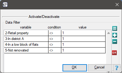
Remember to combine the deactivation conditions with the alternative (replace with ).

As a result, 11 locations were identified ( locations 10, 12, 17, 35, 88, 101, 105, 122, 130, 132, 135) that fit this segment (meeting all 4 conditions).

Now we will consider those features that have a strong influence on the customer's decision, but are not decisive:

Number of rooms = 3;
The floor on which the apartment is located = 0;
Age of the building in which the apartment is located = approx. 3 years;
Proximity of the A district to the city center (time it takes to get to the city center) = approx. 30 min;
Proximity to public transport station = approx. 80 m.

$\begin{tabular}{|c||c|c|c|c|c|} \hline &\textbf{Number of}&\textbf{Apartment}&\textbf{Age of the}&\textbf{Proximity to the}&\textbf{Proximity to the}\\ &\textbf{rooms}&\textbf{floor}&\textbf{building}&\textbf{city center}&\textbf{public transport station}\\\hline\hline \rowcolor[rgb]{0.75,0.75,0.75}Wanted&3&0&3&30&80\\ Lokal 10&2&1&1&0&150\\ Lokal 12&1&2&1&0&200\\ Lokal 17&3&1&7&20&500\\ Lokal 35&2&0&6&5&100\\ Lokal 88&3&4&6&5&200\\ Lokal 101&4&2&10&0&10\\ Lokal 105&2&2&6&0&50\\ Lokal 122&1&0&6&5&100\\ Lokal 130&2&0&10&0&20\\ Lokal 132&3&5&6&30&400\\ Lokal 135&3&1&6&5&100\\ \hline \end{tabular}$

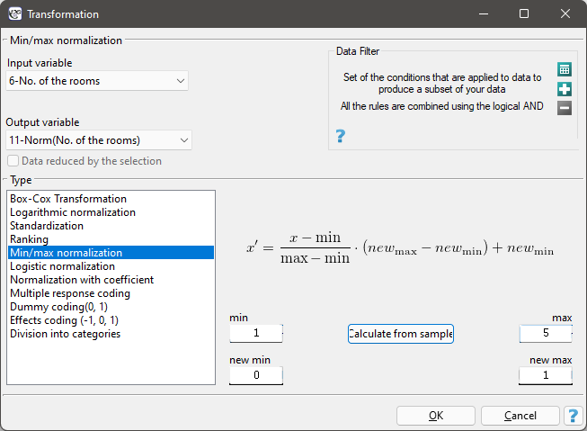
Note that the last feature, the distance of the public transportation station, is expressed by much larger numbers than the other features of the compared locations. As a result, this feature will have a much greater impact on the distance matrix than the other features. To prevent this from happening before the analysis, normalize all the features by choosing a common range from 0 to 1 for them - to do this, use the Data→Normalization/Standardization… menu. In the normalization window, set „Number of rooms” as the input variable and an empty variable called „Norm(Number of rooms)” as the output variable; the normalization type is normalization min/max; the values of min and max are calculated from the sample by selecting the Calculate from sample button - the normalization result will be returned to the datasheet when the Ok button is clicked. The normalization is repeated for the following variables ie: „Floor”, „Building Age”, „Distance to Center” and „Station Distance”.

The normalized data is shown in the table below.

$\begin{tabular}{|c||c|c|c|c|c|} \hline &\footnotesize{\textbf{Norm(Number of}}&\footnotesize{\textbf{Norm(Apartment}}&\footnotesize{\textbf{Norm(Age of the}}&\footnotesize{\textbf{Norm(Proximity to the}}&\footnotesize{\textbf{Norm(Proximity to the}}\\ &\footnotesize{\textbf{rooms)}}&\footnotesize{\textbf{floor)}}&\footnotesize{\textbf{building)}}&\footnotesize{\textbf{city center)}}&\footnotesize{\textbf{public transport station)}}\\\hline\hline \rowcolor[rgb]{0.75,0.75,0.75}Poszukiwany&0,666666667&0&0,222222222&1&0,142857143\\ Lokal 10&0.333333333&0.2&0&0&0.285714286\\ Lokal 12&0&0.4&0&0&0.387755102\\ Lokal 17&0.666666667&0.2&0.666666667&0.666666667&1\\ Lokal 35&0.333333333&0&0.555555556&0.166666667&0.183673469\\ Lokal 88&0.666666667&0.8&0.555555556&0.166666667&0.387755102\\ Lokal 101&1&0.4&1&0&0\\ Lokal 105&0.333333333&0.4&0.555555556&0&0.081632653\\ Lokal 122&0&0&0.555555556&0.166666667&0.183673469\\ Lokal 130&0.333333333&0&1&0&0.020408163\\ Lokal 132&0.666666667&1&0.555555556&1&0.795918367\\ Lokal 135&0.666666667&0.2&0.555555556&0.166666667&0.183673469\\ \hline \end{tabular}$

Based on the normalized data, we will determine the locations that most closely matches the customer's request. To calculate the similarity we will use the Euclidean distance metric. The smaller the value, the more similar the units are. The analysis can be performed assuming that each of the five features mentioned by the client are equally important, but it is also possible to indicate those features that should have greater influence on the result of the analysis. We will construct two Euclidean distance matrices:

[(1)] The first matrix will contain the Euclidean distances calculated from the equivalently treated five features;
[(2)] The second matrix will contain the Euclidean distances, in the construction of which the number of rooms and the distance to the city center will be the most important.

To build the first matrix, in the similarity matrix window, we select 5 normalized variables labeled as Norm, the Euclidean metric, and as Object Identifier the variable „ Location”.

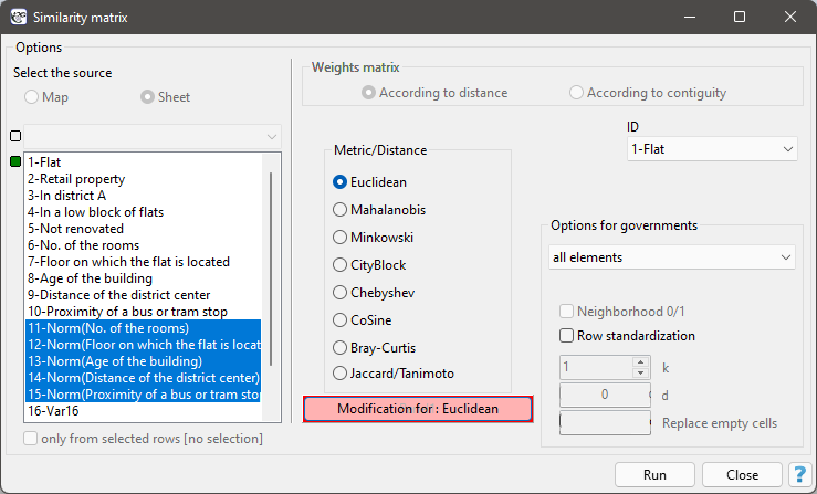
To build the second matrix, we use the same settings in the similarity matrix window as we did to build the first matrix, but in addition, we select the Modification for : Euclidean button and in the modification window, we enter larger values for „Number of rooms” and „Distance to city center”, e.g., equal to 10, and smaller values for the other features, e.g., equal to 1.

This will result in two matrices. In each of them, the first column refers to how similar it is to the location the customer is looking for:

$\begin{tabular}{|c||c|c|} \hline Euclidean&\textbf{Wanted}&...\\\hline \rowcolor[rgb]{0.75,0.75,0.75}Wanted&0&...\\ Location 10&1.10&...\\ Location 12&1.31&...\\ Location 17&1.04&...\\ Location 35&\textcolor[rgb]{0,0,1}{0.96}&...\\ Location 88&1.23&...\\ Location 101&1.38&...\\ Location 105&1.18&...\\ Location 122&1.12&...\\ Location 130&1.32&...\\ Location 132&1.24&...\\ Location 135&\textcolor[rgb]{0,0,1}{0.92}&...\\ \hline \end{tabular}$

$\begin{tabular}{|c||c|c|} \hline Euclidean with scales&\textbf{Wanted}&...\\\hline \rowcolor[rgb]{0.75,0.75,0.75}Wanted&0&...\\ Location 10&3.35&...\\ Location 12&3.84&...\\ Location 17&\textcolor[rgb]{0,0,1}{1.44}&...\\ Location 35&2.86&...\\ Location 88&2.78&...\\ Location 101&3.45&...\\ Location 105&3.37&...\\ Location 122&3.39&...\\ Location 130&3.43&...\\ Location 132&\textcolor[rgb]{0,0,1}{1.24}&...\\ Location 135&2.66&...\\ \hline \end{tabular}$

According to the unmodified Euclidean distance, location 35 and location 135 should most closely match the client's requirements. When the weights are taken into account, locations 17 and 132 are the closest to the client's requirements - these are the locations that are primarily similar in terms of the number of rooms required by the client (3) and the indicated distance to the center, with the other 3 features having a smaller impact on the similarity score.

PQStat - Baza Wiedzy

Narzędzia użytkownika

Narzędzia witryny

Pasek boczny

Similarity matrix

Narzędzia strony