Narzędzia użytkownika
Narzędzia witryny
Pasek boczny
en:statpqpl:usepl:arkpl:normstandpl
Transformations
 The transformation window is accessed via
 Data→Transform…
Data transformation is the alteration of data so that it meets certain criteria, such as meeting the criteria for normality of distribution or extending within a specified range.
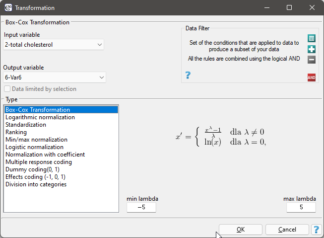
- Box-Cox transformation
The Box-Cox transformation introduced by Box and Cox in 1964 1) brings the data to a normal distribution through a transformation based on the coefficient  . Positive data are required to perform the transformation. If the data are not positive, it is recommended to first transform them to positive numbers using the min-max normalization method.
The Box-Cox transformation is expressed by the formula:

where the value of is determined as the maximum value of the log-likelihood function ( ) in the interval specified by the researcher. The default range for searching for values is the range [-5, 5], and the function is described by the formula:

where:
 - sample size,
 - population standard deviation.
Note
If min-max normalization was used before the Box-Cox transformation, then after the Box-Cox transformation, you can return to the previous range by using this transformation again.
- Logarithmic normalization
The logarithmic transformation can be used to reduce the skewness of the distribution i.e. when we are dealing with a lognormal distribution.

- Standardization
Standardization, is a transformation of data that results in a variable having a mean of 0 and a standard deviation of 1.

- Ranking
Ranks - are consecutive numbers (usually natural) assigned to the values of ordered measurements of the variable under study. They are often used in those nonparametric tests that rely solely on the order of items in the sample. Assigning ranks calculated according to a variable is called ranking. Ranking can be done for variables sorted ascendingly (this is the default setting) or descendingly.
Recurring values of a variable are assigned a tied rank. The tied rank can be a/an:
- arithmetic mean calculated from the proposed consecutive natural numbers for repeated values - this is the default setting;
- lower rank, i.e., the smallest limit proposed for consecutive repeated values of natural numbers;
- the upper rank, meaning the largest proposed for consecutive repeated values of natural numbers.
For example, for a variable with the following values: 8.6, 5.3, 8.6, 7.1, 9.3, 7.2, 7.3, 7.4, 7.3, 5.2, 7, 9.9, 8.6, 5.7 the following ranks are assigned:

While for the variable with a value of 7.3 a tied rank calculated as the arithmetic mean of the numbers:7 and 8 is assigned, and for a variable with value 8.6 a tied rank calculated from the numbers: 10, 11, 12 is assigned.
- Min/max normalization
The min/max normalization through a linear function puts the data into a user-specified range ( ,
,  ). You should know the range that the data can cover. If you do not know the range, you can use the largest and smallest value in the analysed set (in the
 Transformation window, then select the Calculate from sample option)..

- Logistic normalization
Normalization using a logarithmic (S-shaped) function puts the standardized data into the indicated range.
 If you want to stretch the transformed data over a range other than the specified one, then enter the span of the new range in the
 Transformation window.
- Normalizing function with coefficient
This normalization brings the standardized data into the indicated range using an S-shaped function with a changing normalization factor  .
.
 Increasing the value creates a graph with a smoother slope.
- Multiple response coding
This type of coding allows the answers given to multiple-choice questions to be prepared in such a way as to facilitate their further statistical processing. As a result of applying this transformation, a selected variable with  -possible answers is broken down into new variables. It is necessary to specify which character (or set of characters) is a separator of particular categories. For example, respondents were asked what kind of alcohol they drink? The data is stored in Alcohol column, separating multiple answers with semicolon sign. This way of storing data does not even allow for a simple summary. Among other things, it is not possible to quickly count how many people drink wine. After recoding the multiple responses, three new columns were obtained - one for each possible answer. Each of these columns can now be statistically analysed.

- Dummy coding
Transforming a variable with categories by dummy coding allows you to obtain  dummy variables. This form of transformation is primarily used in regression models. A detailed description of this type of transformation can be found in PREPARING VARIABLES FOR ANALYSIS IN MULTI-DIMENSIONAL MODELS.
- Effect coding
Transforming a variable with categories by effect coding yields dummy variables. This form of transformation is used primarily in regression and ANOVA models. A detailed description of this type of transformation can be found in PREPARING VARIABLES FOR ANALYSIS IN MULTI-DIMENSIONAL MODELS.
- Division into categories
This way of preparing data allows for any division of variables, e.g. total cholesterol can be divided according to the current standards (choose Manual division, set the number of categories and enter their limits ourselves and give appropriate labels to each category). However, if we do not have an idea for dividing our data, we can use the automatic division options presented in the window. Possible ways of dividing a variable:
- Natural breaks (Jenks) - a method of dividing a variable into classes such that the variance within classes is minimized and the variance between classes is maximized.
- Division by Quantiles - a method of dividing a variable into classes of equal frequency.
- Standard Deviation - a method of dividing a variable into classes based on its distance from the mean by 1, 2, or more standard deviations.
- Standard error of the mean - a method of dividing a variable into classes based on the distance from the mean by 1, 2, or more standard errors of the mean.
- Manual - a method of dividing a variable into classes according to any division entered manually by the user.
In the division window, it is also possible to select Add color scheme then the column that will store the new data will be color coded according to the indicated scheme.
Example (normalizationa.pqs file)
Perform a transformation on the variables contained in the file:
a) Transform the value of triglycerides using the Box-Cox transformation and then check with the appropriate test whether the data have a normal distribution.
b) Transform the value of triglycerides using the logarithmic transformation and then check with the appropriate test whether the data have a normal distribution.
c) Using min-max normalization, transform the selected variables to the range [0,10].
d) Using logistic normalization, transform the selected variables to the specified range.
e) Using normalization with a coefficient, transform the selected variables to the specified range. Do it several times, changing the value of the coefficient .
f) Standardize all data that are normally distributed.
g) Transform the variable showing how body weight changed during the diet so that it represents a normal distribution.
h) The question about past infectious diseases was a multiple choice question. Prepare the obtained answers to this question so that they can be further statistically processed i.e. record each of the multiple answers in a different column.
i) Prepare the education variable so that it is stored using dummy variables with dummy coding.
j) Prepare the total cholesterol variable by dividing it into 3 classes according to the percentiles (quartiles). Give the created classes labels : „low”, „average”, „high” and choose the color scheme.
1)
Box G. E. , Cox D. R. (1964), An analysis of transformations. Journal of the Royal Statistical Society, Series B 26: 211–252
en/statpqpl/usepl/arkpl/normstandpl.txt · ostatnio zmienione: 2022/02/11 17:59 przez admin
Narzędzia strony
Wszystkie treści w tym wiki, którym nie przyporządkowano licencji, podlegają licencji: CC Attribution-Noncommercial-Share Alike 4.0 International
