PQStat - Baza Wiedzy

Spis treści

Preparation of variables for analysis

Preparation of variables for analysis

Matching groups

Why is group matching done?

There are many answers to this question. Let us use an example of a medical situation.

If we estimate the treatment effect from a fully randomized experiment, then by randomly assigning subjects to the treated and untreated groups we create groups that are similar in terms of possible confounding factors. The similarity of the groups is due to the random assignment itself. In such studies, we can examine the pure (not dependent on confounding factors) effect of the treatment method on the outcome of the experiment. In this case, other than random group matching is not necessary.

The possibility of error arises when the difference in treatment outcome between treated and untreated groups may be due not to the treatment itself, but to a factor that induced people to take part in the treatment. This occurs when randomization is not possible for some reason, such as it is an observational study or for ethical reasons we cannot assign treatment arbitrarily. Artificial group matching may then be applicable. For example, if the people we assign to the treatment group are healthier people and the people who are in the control group are people with more severe disease, then it is not the treatment itself but the condition of the patient before treatment that may affect the outcome of the experiment. When we see such an imbalance of groups, it is good if we can decide to randomize, in this way the probem is solved, because drawing people into groups makes them similar. However, we can imagine another situation. This time the group we are interested in will not be treatment subjects but smokers, and the control group will be non-smokers, and the analyses will aim to show the adverse effect of smoking on the occurrence of lung cancer. Then, in order to test whether smoking does indeed increase the risk of lung cancer, it would be unethical to perform a fully randomized trial because it would mean that people randomly selected to the risk group would be forced to smoke. The solution to this situation is to establish an exposure group, i.e. to select a number of people who already smoke and then to select a control group of non-smokers. The control group should be selected because by leaving the selection to chance we may get a non-smoking group that is younger than the smokers only due to the fact that smoking is becoming less fashionable in our country, so automatically there are many young people among the non-smokers.The control should be drawn from non-smokers, but so that it is as similar as possible to the treatment group.In this way we are getting closer to examining the pure (independent of selected confounding factors such as age) effect of smoking/non-smoking on the outcome of the experiment, which in this case is the occurrence of lung cancer. Such a selection can be made by the matching proposed in the program.

One of the main advantages of investigator-controlled matching is that the control group becomes more similar to the treatment group, but this is also the biggest disadvantage of this method. It is an advantage because our study is looking more and more like a randomized study. In a randomized trial, the treatment and control groups are similar on almost all characteristics, including those we don't study - the random allocation provides us with this similarity. With investigator-controlled matching, the treatment and control groups become similar on only selected characteristics.

Ways of assessing similarity:

The first two methods mentioned are based on matching groups through Propensity Score Matching, PSM. This type of matching was proposed by Rosenbaum and Rubin ¹⁾. In practice, it is a technique for matching a control group (untreated or minimally/standardly treated subjects) to a treatment group on the basis of a probability describing the subjects' propensity to assign treatment depending on the observed associated variables. The probability score describing propensity, called the Propensity Score is a balancing score, so that as a result of matching the control group to the treatment group, the distribution of measured associated variables becomes more similar between treated and untreated subjects. The third method does not determine the probability for each individual, but determines a distance/dissimilarity matrix that indicates the objects that are closest/most similar in terms of multiple selected characteristics.

Methods for determining similarity:

Known probability – the Propensity Score, which is a value between 0 and 1 for each person tested, indicates the probability of being in the treatment group. This probability can be determined beforehand by various methods. For example, in a logistic regression model, through neural networks, or many other methods. If a person in the group from which we draw controls obtains a Propensity Score similar to that obtained by a person in the treatment group, then that person can enter the analysis because the two are similar in terms of the characteristics that were considered in determining the Propensity Score.
Calculated from the logistic regression model – because logistic regression is the most commonly used matching method, PQStat provides the ability to determine a Propensity Score value based on this method automatically in the analysis window. The matching proceeds further using the Propensity Score thus obtained.
Similarity/distance matrix – This option does not determine the value of Propensity Score, but builds a matrix indicating the distance of each person in the treatment group to the person in the control group. The user can set the boundary conditions, e.g. he can indicate that the person matched to a person from the treatment group cannot differ from him by more than 3 years of age and must be of the same sex. Distances in the constructed matrix are determined based on any metric or method describing dissimilarity. This method of matching the control group to the treated group is very flexible. In addition to the arbitrary choice of how the distances/dissimilarity are determined, in many metrics it allows for the indication of weights that determine how important each variable is to the researcher, i.e., the similarity of some variables may be more important to the researcher while the similarity of others is less important. However, great caution is advised when choosing a distance/ dissimilarity matrix. Many features and many sops to determine distances require prior standardization or normalization of the data, moreover, choosing the inverse of distance or similarity (rather than dissimilarity) may result in finding the most distant and dissimilar objects, whereas we normally use these methods to find similar objects. If the researcher does not have specific reasons for changing the metric, the standard recommendation is to use statistical distance, i.e. the Mahalanobia metric – It is the most universal, does not require prior standardization of data and is resistant to correlation of variables. More detailed description of distances and dissimilarity/similarity measures available in the program as well as the method of inetrpratation of the obtained results can be found in the Similarity matrix section .

In practice, there are many methods to indicate how close the objects being compared are, in this case treated and untreated individuals. Two are proposed in the program:

Nearest neighbor method – is a standard way of selecting objects not only with a similar Propensity Score, but also those whose distance/dissimilarity in the matrix is the smallest.
The nearest neighbor method, closer than… – works in the same way as the nearest neighbor method, with the difference that only objects that are close enough can be matched. The limit of this closeness is determined by giving a value describing the threshold, behind which there are already objects so dissimilar to the tested objects, that we do not want to give them a chance to join the newly built control group. In the case when analysis is based on Propensity Score or matrix defined by dissimilarity, the most dissimilar objects are those distant by 1, and the most similar are those distant by 0. Choosing this method we should give a value closer to 0, when we select more restrictively, or closer to 1, when the threshold will be placed further. When we determine distances instead of dissimilarities in the matrix, then the minimum size is also 0, but the maximum size is not predetermined.

We can match without returning already drawn objects or with returning these objects again to the group from which we draw.

Matching without returning – when using no-return matching, once an untreated person has been selected for matching with a given treated person, that untreated person is no longer available for consideration as a potential match for subsequent treated persons. As a result, each untreated individual is included in at most one matching set.
Matching with returning – return matching allows a given untreated individual to be included more than once in a single matched set. When return matching is used, further analyses, and in particular variance estimation, must take into account the fact that the same untreated individual may be in multiple matched sets.

In the case when it is impossible to match the untreated person to the treated one, because in the group from which we choose there are more persons matching the treated one equally well, then one of these persons chosen in a random way is combined. For a renewed analysis, a fixed seed is set by default so that the results of a repeated draw will be the same, but when the analysis is performed again the seed is changed and the result of the draw may be different.

If it is not possible to match an untreated person to a treated one, because there are no more persons to join in the group from which we are choosing, e.g. matching persons have already been joined to other treated persons or the set from which we are choosing has no similar persons, then this person remains without a pair.

Most often a 1:1 match is made,i.e., for one treated person, one untreated person is matched. However, if the original control group from which we draw is large enough and we need to draw more individuals, then we can choose to match 1:k, where k indicates the number of individuals that should be matched to each treated individual.

Matching evaluation

After matching the control group to the treatment group, the results of such matching can be returned to the worksheet, i.e. a new control group can be obtained. However, we should not assume that by applying the matching we will always obtain satisfactory results. In many situations, the group from which we draw does not have a sufficient number of such objects that are sufficiently similar to the treatment group. Therefore, the matching performed should always be evaluated. There are many methods of evaluating the matching of groups. The program uses methods based on standardized group difference and Propensity Score percentile agreement of the treatment group and the control group, more extensively described in the work of P.C Austin, among others ²⁾³⁾. This approach allows comparison of the relative balance of variables measured in different units, and the result is not affected by sample size. The estimation of concordance using statistical tests was abandoned because the matched control group is usually much smaller than the original control group, so that the obtained p-values of tests comparing the test group to the smaller control group are more likely to be left with the null hypothesis, and therefore do not show significant differences due to the reduced size.

For comparison of continuous variables we determine the standardized mean difference:

$\begin{displaymath} d=\frac{\left(\bar{x}_{treated}-\bar{x}_{control}\right)}{\sqrt{\frac{sd^2_{treated}+sd^2_{control}}{2}}} \end{displaymath}$

where:

$\bar{x}_{treated}$ , $\bar{x}_{control}$ – is the mean value of the variable in the treatment group and the mean value of the variable in the control group,

$sd^2_{treated}$ , $sd^2_{control}$ – is the variance in the treatment group and the variance in the control group.

To compare binary variables (of two categories, usually 0 and 1) we determine the standardized frequency difference:

$\begin{displaymath} d=\frac{\left(\hat{p}_{treated}-\hat{p}_{control}\right)}{\sqrt{\frac{\hat{p}_{treated}(1-\hat{p}_{treated})+\hat{p}_{control}(1-\hat{p}_{control})}{2}}} \end{displaymath}$

where:

$\hat{p}_{treated}$ , $\hat{p}_{control}$ – is the frequency of the value described as 1 in the treatment group and the frequency of the value described as 1 in the control group.

Variables with multiple categories we should break down in logistic regression analysis into dummy variables with two categories and, by checking the fits of both groups, determine the standardized frequency difference for them.

Note

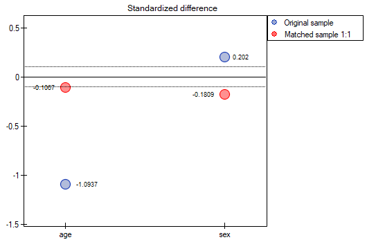
Although there is no universally agreed criterion for what threshold of standardized difference can be used to indicate significant imbalance, a standardized difference of less than 0.1 (in both mean and frequency estimation) can provide a clue ⁴⁾. Therefore, to conclude that the groups are well matched, we should observe standardized differences close to 0, and preferably not outside the range of -0.1 to 0.1. Graphically, these results are presented in a dot plot. Negative differences indicate lower means/frequencies in the treatment group, positive in the control group.

Note

The 1:1 match obtained in the reports means the summary for the study group and the corresponding control group obtained in the first match, the 1:2 match means the summary for the study group and the corresponding control group obtained in the first + second match (i.e., not the study group and the corresponding control group obtained in the second match only), etc.

The window with the settings of group matching options is launched from the menu Advanced statistics→Multivariate models→Propensity Score

EXAMPLE (matching.pqs file)

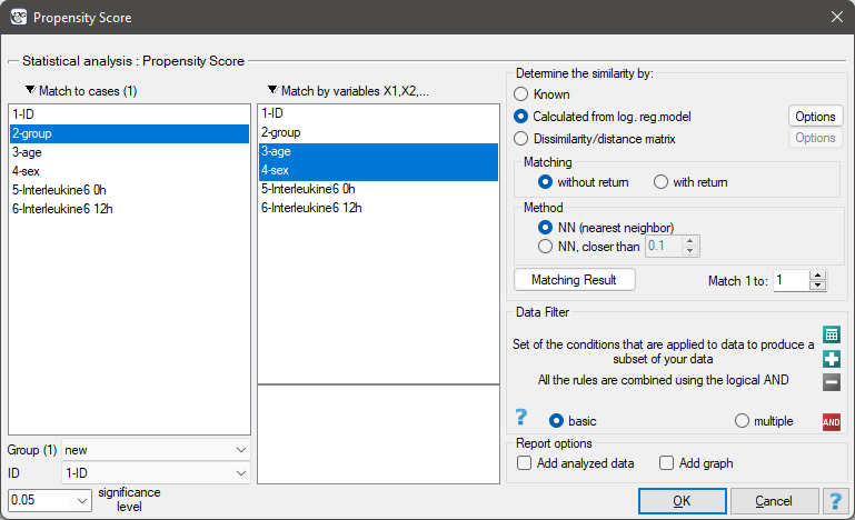
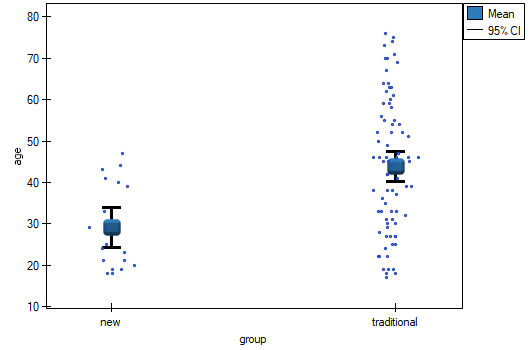
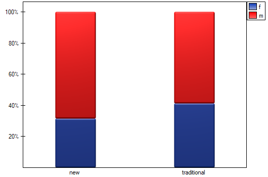
We want to compare two ways of treating patients after accidents, the traditional way and the new one. The correct effect of both treatments should be observed in the decreasing levels of selected cytokines. To compare the effectiveness of the two treatments, they should both be carried out on patients who are quite similar. Then we will be sure that any differences in the effectiveness of these treatments will be due to the treatment effect itself and not to other differences between patients assigned to different groups. The study is a posteriori, that is, it is based on data collected from patients' treatment histories. Therefore, the researchers had no influence on the assignment of patients to the new drug treatment group and the traditional treatment group. It was noted that the traditional treatment was mainly prescribed to older patients, while the new treatment was prescribed to younger patients, in whom it is easier to lower cytokine levels. The groups were fairly similar in gender structure, but not identical.

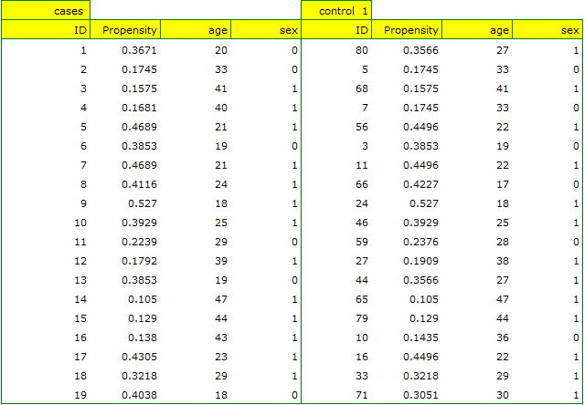
If the planned study had been carried out on such selected groups of patients, the new way would have had an easier challenge, because younger organisms might have responded better to the treatment. The conditions of the experiment would not be equal for both ways, which could falsify the results of the analyses and the conclusions drawn. Therefore, it was decided to match the group treated traditionally to be similar to the study group treated with the new way. We planned to make the matching with respect to two characteristics, i.e. age and gender. The traditional treatment group is larger (80 patients) than the new treatment group (19 patients), so there is a good chance that the groups will be similar. Random selection is performed by the logistic regression model algorithm embedded in the PSM. We remember that gender should be coded numerically, since only numerical values are involved in the logistic regression analysis. We choose nearest neighbor as the method. We want the same person to be unable to be selected duplicately, so we choose a no return randomization. We will try 1:1 matching, i.e. for each person treated with the new drug we will match one person treated traditionally. Remember that the matching is random, so it depends on the random value of seed set by our computer, so the randomization performed by the reader may differ from the values presented here.

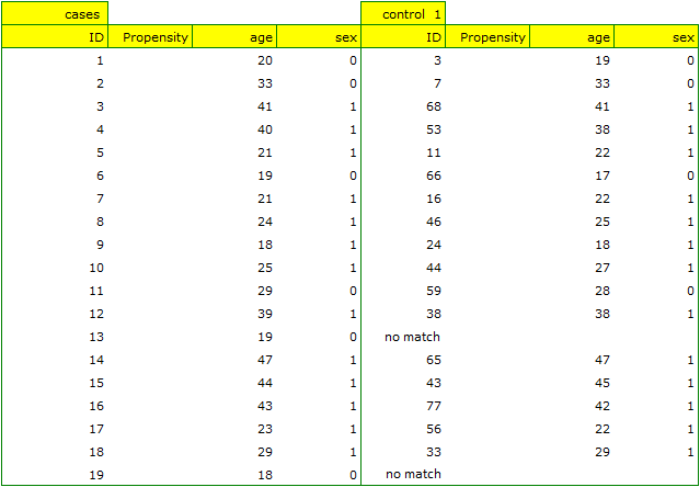
A summary of the selection can be seen in the tables and charts.

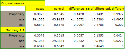
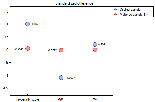
The line at 0 indicates equilibrium of the groups (difference between groups equal to 0). When the groups are in equilibrium with respect to the given characteristics, then all points on the graph are close to this line, i.e., around the interval -0.1 to 0.1. In the case of the original sample (blue color), we see a significant departure of Propensity Score. As we know, this mismatch is mainly due to age mismatch – its standardized difference is at a large distance from 0, and to a lesser extent gender mismatch.

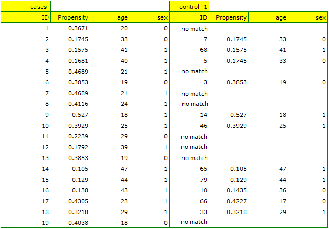
By performing the matching we obtained groups more similar to each other (red color in the graph). The standardized difference between the groups as determined by Propensity Score is 0.0424, which is within the specified range. The age of both groups is already similar – the traditional treatment group differs from the new treatment group by less than a year on average (the difference between the averages presented in the table is 0.2632) and the standardized difference between the averages is -0.0277. In the case of gender, the match is perfect, i.e. the percentage of females and males is the same in both groups (the standardized difference between the percentages presented in the table and the graph is now 0). We can return the data prepared in this way to the worksheet and subject it to the analyses we have planned.

Looking at the summary we just obtained, we can see that despite the good balancing of the groups and the perfect match of many individuals, there are individuals who are not as similar as we might expect.

Sometimes in addition to obtaining well-balanced groups, researchers are interested in determining the exact way of selecting individuals, i.e. obtaining a greater influence on the similarity of objects as to the value of Propensity Score or on the similarity of objects as to the value of specific characteristics. Then, if the group from which we draw is sufficiently large, the analysis may yield results that are more favorable from the researcher's point of view, but if in the group from which we draw there is a lack of objects meeting our criteria, then for some people we will not be able to find a match that meets our conditions.

Suppose that we would like to obtain such groups whose Propensity Score (i.e., propensity to take the survey) differs by no more than …

How to determine this value? You can take a look at the report from the earlier analysis, where the smallest and largest distance between the drawn objects is given.

In our case the objects closest to each other differ by min=0, and the furthest by max=0.5183. We will try to check what kind of selection we will obtain when we will match to people treated with the new method such people treated traditionally, whose Propensity Score will be very close to e.g. less than 0.01.

We can see that this time with failed to select the whole group. Comparing Propensity Score for each pair (treated with the new method and treated traditionally) we can see that the differences are really small. However, since the matched group is much smaller, to sum up the whole process we have to notice that both Propensity Score, age and sex are not close enough to the line at 0. Our will to improve the situation did not lead to the desired effect, and the obtained groups are not well balanced.

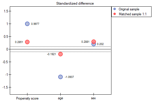
Suppose we wanted to obtain such pairs (subjects treated with the new method and subjects treated traditionally) who are of the same sex and whose ages do not differ by more than 3 years. In the Propensity Score-based randomization, we did not have this type of ability to influence the extent of concordance of each variable. For this we will use a different method, not based on Propensity Score, but based on distance/dissimilarity matrices. After selecting the Options button, we select the proposed Mahalanobis statistical distance matrix and set the neighborhood fit to a maximum distance equal to 3 for age and equal to 0 for gender. As a result, for two people we failed to find a match, but the remaining matches meet the set criteria.

To summarize the overall draw, we note that although it meets our assumptions, the resulting groups are not as well balanced as they were in our first draw based on Propensity Score. The points in red representing the quality of the match by age and the quality of the match by gender deviate slightly from the line of sameness set at level 0, which means that the average difference in age and sex structure is now greater than in the first matching.

It is up to the researcher to decide which way of preparing the data will be more beneficial to them.

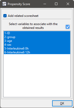
Finally, when the decision is made, the data can be returned to a new worksheet. To do this, go back to the report you selected and in the project tree under the right button select the Redo analysis menu. In the same analysis window, point to the Fit Result button and specify which other variables will be returned to the new worksheet.

This will result in a new data sheet with side-by-side data for people treated with the new treatment and matched people treated traditionally.

2022/02/26 15:35 · admin

Interctions

Interactions are considered in multidimensional models. Their presence means that the influence of the independent variable ( $X_1$ ) on the dependent variable ( $Y$ ) differs depending on the level of another independent variable ( $X_2$ ) or a series of other independent variables. To discuss the interactions in multidimensional models one must determine the variables informing about possible interactions, i.e the product of appropriate variables. For that purpose we select the Interactions button in the window of the selected multidimensional analysis. In the window of interactions settings, with the CTRL button pressed, we determine the variables which are to form interactions and transfer the variables into the neighboring list with the use of an arrow. By pressing the OK button we will obtain appropriate columns in the datasheet.

In the analysis of the interaction the choice of appropriate coding of dichotomous variables allows the avoidance of the over-parametrization related to interactions. Over-parametrization causes the effects of the lower order for dichotomous variables to be redundant with respect to the confounding interactions of the higher order. As a result, the inclusion of the interactions of the higher order in the model annuls the effect of the interactions of the lower orders, not allowing an appropriate evaluation of the latter. In order to avoid the over-parametrization in a model in which there are interactions of dichotomous variables it is recommended to choose the option effect coding.

In models with interactions, remember to „trim” them appropriately, so that when removing the main effects, we also remove the effects of higher orders that depend on them. That is: if in a model we have the following variables (main effects): $X_1$ , $X_2$ , $X_3$ and interactions: $X_1*X_2$ , $X_1*X_3$ , $X_2*X_3$ , $X_1*X_2*X_3$ , then by removing the variable $X_1$ from the model we must also remove the interactions in which it occurs, viz: $X_1*X_2$ , $X_1*X_3$ and $X_1*X_2*X_3$ .

2022/02/09 12:56

Variables coding

When preparing data for a multidimensional analysis there is the problem of appropriate coding of nominal and ordinal variables. That is an important element of preparing data for analysis as it is a key factor in the interpretation of the coefficients of a model. The nominal or ordinal variables divide the analyzed objects into two or more categories. The dichotomous variables (in two categories, $k=2$ ) must only be appropriately coded, whereas the variables with many categories ( $k>2$ ) ought to be divided into dummy variables with two categories and coded.

[ $k=2$ ] If a variable is dichotomous, it is the decision of the researcher how the data representing the variable will be entered, so any numerical codes can be entered, e.g. 0 and 1. In the program one can change one's coding into effect coding by selecting that option in the window of the selected multidimensional analysis. Such coding causes a replacement of the smaller value with value -1 and of the greater value with value 1.
[ $k>2$ ] If a variable has many categories then in the window of the selected multidimensional analysis we select the button Dummy variables and set the reference/base category for those variables which we want to break into dummy variables. The variables will be dummy coded unless the effect coding option will be selected in the window of the analysis – in such a case, they will be coded as -1, 0, and 1.

Dummy coding is employed in order to answer, with the use of multidimensional models, the question: How do the ( $Y$ ) results in any analyzed category differ from the results of the reference category. The coding consists in ascribing value 0 or 1 to each category of the given variable. The category coded as 0 is, then, the reference category.

[ $k=2$ ] If the coded variable is dichotomous, then by placing it in a regression model we will obtain the coefficient calculated for it, ( $b_i$ ). The coefficient is the reference of the value of the dependent variable $Y$ for category 1 to the reference category (corrected with the remaining variables in the model).
[ $k>2$ ] If the analyzed variable has more than two categories, then $k$ categories are represented by $k-1$ dummy variables with dummy coding. When creating variables with dummy coding one selects a category for which no dummy category is created. That category is treated as a reference category (as the value of each variable coded in the dummy coding is equal to 0.

When the $X_1, X_2, ..., X_{k-1}$ variables obtained in that way, with dummy coding, are placed in a regression model, then their $b_1, b_2, ..., b_{k-1}$ coefficients will be calculated.

[ $b_1$ ] is the reference of the $Y$ results (for codes 1 in $X_1$ ) to the reference category (corrected with the remaining variables in the model);
[ $b_2$ ] is the reference of the $Y$ results (for codes 1 in $X_2$ ) to the reference category (corrected with the remaining variables in the model);
[…]
[ $b_{k-1}$ ] is the reference of the $Y$ results (for codes 1 in $X_{k-1}$ ) to the reference category (corrected with the remaining variables in the model);

Example

We code, in accordance with dummy coding, the sex variable with two categories (the male sex will be selected as the reference category), and the education variable with 4 categories (elementary education will be selected as the reference category).

$\mbox{\begin{tabular}{|c|c|} \hline &\textcolor[rgb]{0.5,0,0.5}{\textbf{Coded}}\\ \textbf{Sex}&\textcolor[rgb]{0.5,0,0.5}{\textbf{sex}}\\\hline f&\textcolor[rgb]{0.5,0,0.5}{1}\\ f&\textcolor[rgb]{0.5,0,0.5}{1}\\ f&\textcolor[rgb]{0.5,0,0.5}{1}\\ \cellcolor[rgb]{0.88,0.88,0.88}m&\cellcolor[rgb]{0.88,0.88,0.88}0\\ \cellcolor[rgb]{0.88,0.88,0.88}m&\cellcolor[rgb]{0.88,0.88,0.88}0\\ f&\textcolor[rgb]{0.5,0,0.5}{1}\\ f&\textcolor[rgb]{0.5,0,0.5}{1}\\ \cellcolor[rgb]{0.88,0.88,0.88}m&\cellcolor[rgb]{0.88,0.88,0.88}0\\ \cellcolor[rgb]{0.88,0.88,0.88}m&\cellcolor[rgb]{0.88,0.88,0.88}0\\ f&\textcolor[rgb]{0.5,0,0.5}{1}\\ \cellcolor[rgb]{0.88,0.88,0.88}m&\cellcolor[rgb]{0.88,0.88,0.88}0\\ f&\textcolor[rgb]{0.5,0,0.5}{1}\\ \cellcolor[rgb]{0.88,0.88,0.88}m&\cellcolor[rgb]{0.88,0.88,0.88}0\\ f&\textcolor[rgb]{0.5,0,0.5}{1}\\ \cellcolor[rgb]{0.88,0.88,0.88}m&\cellcolor[rgb]{0.88,0.88,0.88}0\\ \cellcolor[rgb]{0.88,0.88,0.88}m&\cellcolor[rgb]{0.88,0.88,0.88}0\\ ...&...\\\hline \end{tabular}$

$\mbox{\begin{tabular}{|c|ccc|} \hline & \multicolumn{3}{c|}{\textbf{Coded education}}\\ \textbf{Education}&\textcolor[rgb]{0,0,1}{\textbf{vocational}}&\textcolor[rgb]{1,0,0}{\textbf{secondary}}&\textcolor[rgb]{0,0.58,0}{\textbf{tertiary}}\\\hline \cellcolor[rgb]{0.88,0.88,0.88}elementary&\cellcolor[rgb]{0.88,0.88,0.88}0&\cellcolor[rgb]{0.88,0.88,0.88}0&\cellcolor[rgb]{0.88,0.88,0.88}0\\ \cellcolor[rgb]{0.88,0.88,0.88}elementary&\cellcolor[rgb]{0.88,0.88,0.88}0&\cellcolor[rgb]{0.88,0.88,0.88}0&\cellcolor[rgb]{0.88,0.88,0.88}0\\ \cellcolor[rgb]{0.88,0.88,0.88}elementary&\cellcolor[rgb]{0.88,0.88,0.88}0&\cellcolor[rgb]{0.88,0.88,0.88}0&\cellcolor[rgb]{0.88,0.88,0.88}0\\ \textcolor[rgb]{0,0,1}{vocational}&\textcolor[rgb]{0,0,1}{1}&0&0\\ \textcolor[rgb]{0,0,1}{vocational}&\textcolor[rgb]{0,0,1}{1}&0&0\\ \textcolor[rgb]{0,0,1}{vocational}&\textcolor[rgb]{0,0,1}{1}&0&0\\ \textcolor[rgb]{0,0,1}{vocational}&\textcolor[rgb]{0,0,1}{1}&0&0\\ \textcolor[rgb]{1,0,0}{secondary}&0&\textcolor[rgb]{1,0,0}{1}&0\\ \textcolor[rgb]{1,0,0}{secondary}&0&\textcolor[rgb]{1,0,0}{1}&0\\ \textcolor[rgb]{1,0,0}{secondary}&0&\textcolor[rgb]{1,0,0}{1}&0\\ \textcolor[rgb]{1,0,0}{secondary}&0&\textcolor[rgb]{1,0,0}{1}&0\\ \textcolor[rgb]{0,0.58,0}{tertiary}&0&0&\textcolor[rgb]{0,0.58,0}{1}\\ \textcolor[rgb]{0,0.58,0}{tertiary}&0&0&\textcolor[rgb]{0,0.58,0}{1}\\ \textcolor[rgb]{0,0.58,0}{tertiary}&0&0&\textcolor[rgb]{0,0.58,0}{1}\\\ \textcolor[rgb]{0,0.58,0}{tertiary}&0&0&\textcolor[rgb]{0,0.58,0}{1}\\ \textcolor[rgb]{0,0.58,0}{tertiary}&0&0&\textcolor[rgb]{0,0.58,0}{1}\\ ...&...&...&...\\\hline \end{tabular}$

Building on the basis of dummy variables, in a multiple regression model, we might want to check what impact the variables have on a dependent variable, e.g. $Y$ = the amount of earnings (in thousands of PLN). As a result of such an analysis we will obtain sample coefficients for each dummy variable:

- for sex the statistically significant coefficient $b_{i}=-0.5$ , which means that average women's wages are a half of a thousand PLN lower than men's wages, assuming that all other variables in the model remain unchanged;

- for vocational education the statistically significant coefficient $b_{i}=0.6$ , which means that the average wages of people with elementary education are 0.6 of a thousand PLN higher than those of people with elementary education, assuming that all other variables in the model remain unchanged;

- for secondary education the statistically significant coefficient $b_{i}=1$ , which means that the average wages of people with secondary education are a thousand PLN higher than those of people with elementary education, assuming that all other variables in the model remain unchanged;

- for tertiary-level education the statistically significant coefficient $b_{i}=1.5$ , which means that the average wages of people with tertiary-level education are 1.5 PLN higher than those of people with elementary education, assuming that all other variables in the model remain unchanged;

Effect coding is used to answer, with the use of multidimensional models, the question: How do ( $Y$ ) results in each analyzed category differ from the results of the (unweighted) mean obtained from the sample. The coding consists in ascribing value -1 or 1 to each category of the given variable. The category coded as -1 is then the base category

[ $k=2$ ] If the coded variable is dichotomous, then by placing it in a regression model we will obtain the coefficient calculated for it, ( $b_i$ ). The coefficient is the reference of $Y$ for category 1 to the unweighted general mean (corrected with the remaining variables in the model).
If the analyzed variable has more than two categories, then $k$ categories are represented by $k-1$ dummy variables with effect coding. When creating variables with effect coding a category is selected for which no separate variable is made. The category is treated in the models as a base category (as in each variable made by effect coding it has values -1).

When the $X_1, X_2, ..., X_{k-1}$ variables obtained in that way, with effect coding, are placed in a regression model, then their $b_1, b_2, ..., b_{k-1}$ coefficients will be calculated.

[ $b_1$ ] is the reference of the $Y$ results (for codes 1 in $X_1$ ) to the unweighted general mean (corrected by the remaining variables in the model);
[ $b_2$ ] is the reference of the $Y$ results (for codes 1 in $X_2$ ) to the unweighted general mean (corrected by the remaining variables in the model);
[…]
[ $b_{k-1}$ ] is the reference of the $Y$ results (for codes 1 in $X_{k-1}$ ) to the unweighted general mean (corrected by the remaining variables in the model);

Example

With the use of effect coding we will code the sex variable with two categories (the male category will be the base category) and a variable informing about the region of residence in the analyzed country. 5 regions were selected: northern, southern, eastern, western, and central. The central region will be the base one.

$\mbox{\begin{tabular}{|c|c|} \hline &\textcolor[rgb]{0.5,0,0.5}{\textbf{Coded}}\\ \textbf{Sex}&\textcolor[rgb]{0.5,0,0.5}{\textbf{sex}}\\\hline f&\textcolor[rgb]{0.5,0,0.5}{1}\\ f&\textcolor[rgb]{0.5,0,0.5}{1}\\ f&\textcolor[rgb]{0.5,0,0.5}{1}\\ \cellcolor[rgb]{0.88,0.88,0.88}m&\cellcolor[rgb]{0.88,0.88,0.88}-1\\ \cellcolor[rgb]{0.88,0.88,0.88}m&\cellcolor[rgb]{0.88,0.88,0.88}-1\\ f&\textcolor[rgb]{0.5,0,0.5}{1}\\ f&\textcolor[rgb]{0.5,0,0.5}{1}\\ \cellcolor[rgb]{0.88,0.88,0.88}m&\cellcolor[rgb]{0.88,0.88,0.88}-1\\ \cellcolor[rgb]{0.88,0.88,0.88}m&\cellcolor[rgb]{0.88,0.88,0.88}-1\\ f&\textcolor[rgb]{0.5,0,0.5}{1}\\ \cellcolor[rgb]{0.88,0.88,0.88}m&\cellcolor[rgb]{0.88,0.88,0.88}-1\\ f&\textcolor[rgb]{0.5,0,0.5}{1}\\ \cellcolor[rgb]{0.88,0.88,0.88}m&\cellcolor[rgb]{0.88,0.88,0.88}-1\\ f&\textcolor[rgb]{0.5,0,0.5}{1}\\ \cellcolor[rgb]{0.88,0.88,0.88}m&\cellcolor[rgb]{0.88,0.88,0.88}-1\\ \cellcolor[rgb]{0.88,0.88,0.88}m&\cellcolor[rgb]{0.88,0.88,0.88}-1\\ ...&...\\\hline \end{tabular}$

$\mbox{\begin{tabular}{|c|cccc|} \hline \textbf{Regions}& \multicolumn{4}{c|}{\textbf{Coded regions}}\\ \textbf{of residence}&\textcolor[rgb]{0,0,1}{\textbf{western}}&\textcolor[rgb]{1,0,0}{\textbf{eastern}}&\textcolor[rgb]{0,0.58,0}{\textbf{northern}}&\textcolor[rgb]{0.55,0,0}{\textbf{southern}}\\\hline \cellcolor[rgb]{0.88,0.88,0.88}central&\cellcolor[rgb]{0.88,0.88,0.88}-1&\cellcolor[rgb]{0.88,0.88,0.88}-1&\cellcolor[rgb]{0.88,0.88,0.88}-1&\cellcolor[rgb]{0.88,0.88,0.88}-1\\ \cellcolor[rgb]{0.88,0.88,0.88}central&\cellcolor[rgb]{0.88,0.88,0.88}-1&\cellcolor[rgb]{0.88,0.88,0.88}-1&\cellcolor[rgb]{0.88,0.88,0.88}-1&\cellcolor[rgb]{0.88,0.88,0.88}-1\\ \cellcolor[rgb]{0.88,0.88,0.88}central&\cellcolor[rgb]{0.88,0.88,0.88}-1&\cellcolor[rgb]{0.88,0.88,0.88}-1&\cellcolor[rgb]{0.88,0.88,0.88}-1&\cellcolor[rgb]{0.88,0.88,0.88}-1\\ \textcolor[rgb]{0,0,1}{western}&\textcolor[rgb]{0,0,1}{1}&0&0&0\\ \textcolor[rgb]{0,0,1}{western}&\textcolor[rgb]{0,0,1}{1}&0&0&0\\ \textcolor[rgb]{0,0,1}{western}&\textcolor[rgb]{0,0,1}{1}&0&0&0\\ \textcolor[rgb]{0,0,1}{western}&\textcolor[rgb]{0,0,1}{1}&0&0&0\\ \textcolor[rgb]{1,0,0}{eastern}&0&\textcolor[rgb]{1,0,0}{1}&0&0\\ \textcolor[rgb]{1,0,0}{eastern}&0&\textcolor[rgb]{1,0,0}{1}&0&0\\ \textcolor[rgb]{1,0,0}{eastern}&0&\textcolor[rgb]{1,0,0}{1}&0&0\\ \textcolor[rgb]{1,0,0}{eastern}&0&\textcolor[rgb]{1,0,0}{1}&0&0\\ \textcolor[rgb]{0,0.58,0}{northern}&0&0&\textcolor[rgb]{0,0.58,0}{1}&0\\ \textcolor[rgb]{0,0.58,0}{northern}&0&0&\textcolor[rgb]{0,0.58,0}{1}&0\\ \textcolor[rgb]{0.55,0,0}{southern}&0&0&0&\textcolor[rgb]{0.55,0,0}{1}\\ \textcolor[rgb]{0.55,0,0}{southern}&0&0&0&\textcolor[rgb]{0.55,0,0}{1}\\ \textcolor[rgb]{0.55,0,0}{southern}&0&0&0&\textcolor[rgb]{0.55,0,0}{1}\\ ...&...&...&...&...\\\hline \end{tabular}$

Building on the basis of dummy variables, in a multiple regression model, we might want to check what impact the variables have on a dependent variable, e.g. $Y$ = the amount of earnings (expressed in thousands of PLN). As a result of such an analysis we will obtain sample coefficients for each dummy variable:

- for sex the statistically significant coefficient $b_{i}=-0.5$ , which means that the average women's wages are a half of a thousand PLN lower than the average wages in the country, assuming that the other variables in the model remain unchanged;

- for the western region the statistically significant coefficient $b_{i}=0.6$ , which means that the average wages of people living in the western region of the country are 0.6 thousand PLN higher than the average wages in the country, assuming that the other variables in the model remain unchanged;

- for the eastern region the statistically significant coefficient $b_{i}=-1$ , which means that the average wages of people living in the eastern region of the country are a thousand PLN lower than the average wages in the country, assuming that the other variables in the model remain unchanged;

- for the northern region the statistically significant coefficient $b_{i}=0.4$ , which means that the average wages of people living in the western region of the country are 0.4 thousand PLN higher than the average wages in the country, assuming that the other variables in the model remain unchanged;

- for the southern region the statistically significant coefficient $b_{i}=0.1$ , which means that the average wages of people living in the southern region of the country do not differ in a statistically significant manner from the average wages in the country, assuming that the other variables in the model remain unchanged;

2022/02/09 12:56

¹⁾

Rosenbaum P.R., Rubin D.B. (1983a), The central role of the propensity score in observational studies for causal effects. Biometrika; 70:41–55

²⁾

Austin P.C., (2009), The relative ability of different propensity score methods to balance measured covariates between treated and untreated subjects in observational studies. Med Decis Making; 29(6):661-77

³⁾

Austin P.C., (2011), An Introduction to Propensity Score Methods for Reducing the Effects of Confounding in Observational Studies. Multivariate Behavioral Research 46, 3: 399–424

⁴⁾

Normand S.L. T., Landrum M.B., Guadagnoli E., Ayanian J.Z., Ryan T.J., Cleary P.D., McNeil B.J. (2001), Validating recommendations for coronary angiography following an acute myocardial infarction in the elderly: A matched analysis using propensity scores. Journal of Clinical Epidemiology; 54:387–398.

PQStat - Baza Wiedzy

Narzędzia użytkownika

Narzędzia witryny

Pasek boczny

Spis treści

Preparation of variables for analysis

Matching groups

Interctions

Variables coding

Narzędzia strony