PQStat - Baza Wiedzy

Spis treści

Logistic regression

Logistic regression

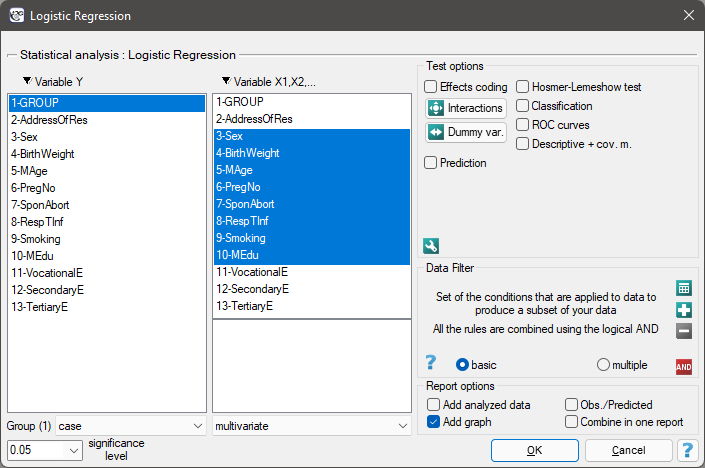
The window with settings for Logistic Regression is accessed via the menu Advanced statistics→Multidimensional Models→Logistic Regression

The constructed model of logistic regression (similarly to the case of multiple linear regression) allows the study of the effect of many independent variables ( $X_1, X_2,..., X_k$ ) on one dependent variable( $Y$ ). This time, however, the dependent variable only assumes two values, e.g. ill/healthy, insolvent/solvent etc.

The two values are coded as (1)/(0), where:

(1) the distinguished value - possessing the feature

(0) not possessing the feature.

The function on which the model of logistic regression is based does not calculate the 2-level variable $Y$ but the probability of that variable assuming the distinguished value:

$\begin{displaymath} P(Y=1|X_1,X_2,...,X_k)=\frac{e^Z}{1+e^Z} \end{displaymath}$

where:

$P(Y=1|X_1,X_2,...,X_k)$ - the probability of assuming the distinguished value (1) on condition that specific values of independent variables are achieved, the so-called probability predicted for 1.

$Z$ is most often expressed in the form of a linear relationship:

$Z=\beta_0+\sum_{i=1}^k\beta_iX_i$ ,

$X_1,X_2,\ldots X_k$ - independent variables, explanatory,

$\beta_0,\beta_1,\beta_2,\ldots \beta_k$ - parameters.

Dummy variables and interactions in the model

A discussion of the coding of dummy variables and interactions is presented in chapter Preparation of the variables for the analysis in multidimensional models.

Note Function Z can also be described with the use of a higher order relationship, e.g. a square relationship - in such a case we introduce into the model a variable containing the square of the independent variable $X_i^2$ .

The logit is the transformation of that model into the form:

$\begin{displaymath} \ln\left(\frac{P}{1-P}\right)=Z. \end{displaymath}$

The matrices involved in the equation, for a sample of size $n$ , are recorded in the following manner:

$Y=\left( \begin{array}{ccc} y_1\\ y_2\\ \vdots\\ y_n \end{array} \right),$

$X=\left( \begin{array}{ccccc} 1 & x_{11} & x_{21} & \ldots & x_{k1}\\ 1 & x_{12} & x_{22} & \ldots & x_{k2}\\ \vdots & \vdots & \vdots & \ddots & \vdots\\ 1 & x_{1n} & x_{2n} & \ldots & x_{kn} \end{array} \right),$

$\beta=\left( \begin{array}{ccc} \beta_0\\ \beta_1\\ \beta_2\\ \vdots\\ \beta_k \end{array} \right).$

In such a case, the solution of the equation is the vector of the estimates of parameters $\beta_0,\beta_1,\ldots,\beta_k$ called regression coefficients:

$b=\left( \begin{array}{ccc} b_0\\ b_1\\ b_2\\ \vdots\\ b_k \end{array} \right).$

The coefficients are estimated with the use of the maximum likelihood method, that is through the search for the maximum value of likelihood function $L$ (in the program the Newton-Raphson iterative algorithm was used). On the basis of those values we can infer the magnitude of the effect of the independent variable (for which the coefficient was estimated) on the dependent variable.

There is a certain error of estimation for each coefficient. The magnitude of that error is estimated from the following formula:

$\begin{displaymath} SE_b=\sqrt{diag(H^{-1})_b}, \end{displaymath}$

where:

$diag(H^{-1})$ is the main diagonal of the covariance matrix.

Note When building the model you need remember that the number of observations should be ten times greater than or equal to the number of the estimated parameters of the model ( $n\ge 10(k+1)$ ). However, a more restrictive criterion proposed by P. Peduzzi et al. in 1996¹⁾ is increasingly used, stating that the number of observations should be ten times or equal to the ratio of the number of independent variables ( $v$ ) and the smaller of the proportion of counts ( $p$ )described from the dependent variable (i.e., proportions of sick or healthy), i.e. ( $n\ge 10v/p$ ).

Note When building the model you need remember that the independent variables should not be collinear. In a case of collinearity estimation can be uncertain and the obtained error values very high. The collinear variables should be removed from the model or one independent variable should be built of them, e.g. instead of the collinear variables of mother age and father age one can build the parents age variable.

Note The criterion of convergence of the function of the Newton-Raphson iterative algorithm can be controlled with the help of two parameters: the limit of convergence iteration (it gives the maximum number of iterations in which the algorithm should reach convergence) and the convergence criterion (it gives the value below which the received improvement of estimation shall be considered to be insignificant and the algorithm will stop).

The Odds Ratio

Individual Odds Ratio

On the basis of many coefficients, for each independent variable in the model an easily interpreted measure is estimated, i.e. the individual Odds Ratio: $\begin{displaymath} OR_i=e^{\beta_i}. \end{displaymath}$

The received Odds Ratio expresses the change of the odds for the occurrence of the distinguished value (1) when the independent variable grows by 1 unit. The result is corrected with the remaining independent variables in the model so that it is assumed that they remain at a stable level while the studied variable is growing by 1 unit.

The OR value is interpreted as follows:

$OR >1$ means the stimulating influence of the studied independent variable on obtaining the distinguished value (1), i.e. it gives information about how much greater are the odds of the occurrence of the distinguished value (1) when the independent variable grows by 1 unit.
$OR <1$ means the destimulating influence of the studied independent variable on obtaining the distinguished value (1), i.e. it gives information about how much lower are the odds of the occurrence of the distinguished value (1) when the independent variable grows by 1 unit.
$OR\approx1$ means that the studied independent variable has no influence on obtaining the distinguished value (1).

Odds Ratio - the general formula

The PQStat program calculates the individual Odds Ratio. Its modification on the basis of a general formula makes it possible to change the interpretation of the obtained result.

The Odds Ratio for the occurrence of the distinguished state in a general case is calculated as the ratio of two odds. Therefore for the independent variable $X_1$ for $Z$ expressed with a linear relationship we calculate:

the odds for the first category: $\begin{displaymath} Odds(1)=\frac{P(1)}{1-P(1)}=e^Z(1)=e^{\beta_0+\beta_1X_1(1)+\beta_2X_2+...+\beta_kX_k}, \end{displaymath}$

the odds for the second category:

$\begin{displaymath} Odds(2)=\frac{P(2)}{1-P(2)}=e^Z(2)=e^{\beta_0+\beta_1X_1(2)+\beta_2X_2+...+\beta_kX_k}. \end{displaymath}$

The Odds Ratio for variable $X_1$ is then expressed with the formula:

$\begin{displaymath} \begin{array}{lll} OR_1(2)/(1) &=&\frac{Odds(2)}{Odds(1)}=\frac{e^{\beta_0+\beta_1X_1(2)+\beta_2X_2+...+\beta_kX_k}}{e^{\beta_0+\beta_1X_1(1)+\beta_2X_2+...+\beta_kX_k}}\\ &=& e^{\beta_0+\beta_1X_1(2)+\beta_2X_2+...+\beta_kX_k-[\beta_0+\beta_1X_1(1)+\beta_2X_2+...+\beta_kX_k]}\\ &=& e^{\beta_1X_1(2)-\beta_1X_1(1)}=e^{\beta_1[X_1(2)-X_1(1)]}=\\ &=& \left(e^{\beta_1}\right)^{[X_1(2)-X_1(1)]}. \end{array} \end{displaymath}$

Example

If the independent variable is age expressed in years, then the difference between neighboring age categories such as 25 and 26 years is 1 year $\left(X_1(2)-X_1(1)=26-25=1\right)$ . In such a case we will obtain the individual Odds Ratio:

$\begin{displaymath}OR=\left(e^{\beta_1}\right)^1,\end{displaymath}$

which expresses the degree of change of the odds for the occurrence of the distinguished value if the age is changed by 1 year.

The odds ratio calculated for non-neighboring variable categories, such as 25 and 30 years, will be a five-year Odds Ratio, because the difference $X_1(2)-X_1(1)=30-25=5$ . In such a case we will obtain the five-year Odds Ratio:

$\begin{displaymath}OR=\left(e^{\beta_1}\right)^5,\end{displaymath}$

which expresses the degree of change of the odds for the occurrence of the distinguished value if the age is changed by 5 years.

Note

If the analysis is made for a non-linear model or if interaction is taken into account, then, on the basis of a general formula, we can calculate an appropriate Odds Ratio by changing the formula which expresses $Z$ .

EXAMPLE cont. (task.pqs file)

EXAMPLE cont. (anomaly.pqs file)

2022/02/09 12:56

Model verification

Statistical significance of particular variables in the model (significance of the Odds Ratio)

On the basis of the coefficient and its error of estimation we can infer if the independent variable for which the coefficient was estimated has a significant effect on the dependent variable. For that purpose we use Wald test.

Hypotheses:

$\begin{array}{cc} \mathcal{H}_0: & \beta_i=0,\\ \mathcal{H}_1: & \beta_i\ne 0. \end{array}$

or, equivalently:

$\begin{array}{cc} \mathcal{H}_0: & OR_i=1,\\ \mathcal{H}_1: & OR_i\ne 1. \end{array}$

The Wald test statistics is calculated according to the formula:

$\begin{displaymath} \chi^2=\left(\frac{b_i}{SE_{b_i}}\right)^2 \end{displaymath}$

The statistic asymptotically (for large sizes) has the Chi-square distribution with $1$ degree of freedom.

The p-value, designated on the basis of the test statistic, is compared with the significance level $\alpha$ :

$\begin{array}{ccl} $ if $ p \le \alpha & \Longrightarrow & $ reject $ \mathcal{H}_0 $ and accept $ \mathcal{H}_1, \\ $ if $ p > \alpha & \Longrightarrow & $ there is no reason to reject $ \mathcal{H}_0. \\ \end{array}$

The quality of the constructed model

A good model should fulfill two basic conditions: it should fit well and be possibly simple. The quality of multiple linear regression can be evaluated can be evaluated with a few general measures based on: $L_{FM}$ - the maximum value of likelihood function of a full model (with all variables),

$L_0$ - the maximum value of the likelihood function of a model which only contains one free word,

$n$ - the sample size.

Information criteria are based on the information entropy carried by the model (model insecurity), i.e. they evaluate the lost information when a given model is used to describe the studied phenomenon. We should, then, choose the model with the minimum value of a given information criterion.

$AIC$ , $AICc$ , and $BIC$ is a kind of a compromise between the good fit and complexity. The second element of the sum in formulas for information criteria (the so-called penalty function) measures the simplicity of the model. That depends on the number of variables ( $k$ ) in the model and the sample size ( $n$ ). In both cases the element grows with the increase of the number of variables and the growth is the faster the smaller the number of observations. The information criterion, however, is not an absolute measure, i.e. if all the compared models do not describe reality well, there is no use looking for a warning in the information criterion.

Akaike information criterion

$\begin{displaymath} AIC=-2\ln L_{FM}+2k, \end{displaymath}$

It is an asymptomatic criterion, appropriate for large sample sizes.

Corrected Akaike information criterion

$\begin{displaymath} AICc=AIC+\frac{2k(k+1)}{n-k-1}, \end{displaymath}$

Because the correction of the Akaike information criterion concerns the sample size it is the recommended measure (also for smaller sizes).

Bayesian information criterion or Schwarz criterion

$\begin{displaymath} BIC=-2\ln L_{FM}+k\ln(n), \end{displaymath}$

Just like the corrected Akaike criterion it takes into account the sample size.

Pseudo R $^2$ - the so-called McFadden R $^2$ is a goodness of fit measure of the model (an equivalent of the coefficient of multiple determination $R^2$ defined for multiple linear regression).

The value of that coefficient falls within the range of $<0; 1)$ , where values close to 1 mean excellent goodness of fit of a model, $0$ - a complete lack of fit Coefficient $R^2_{Pseudo}$ is calculated according to the formula:

$\begin{displaymath} R^2_{Pseudo}=1-\frac{\ln L_{FM}}{\ln L_0}. \end{displaymath}$

As coefficient $R^2_{Pseudo}$ never assumes value 1 and is sensitive to the amount of variables in the model, its corrected value is calculated:

$\begin{displaymath} R^2_{Nagelkerke}=\frac{1-e^{-(2/n)(\ln L_{FM}-\ln L_0)}}{1-e^{(2/n)\ln L_0}} \quad \textrm{lub}\quad R^2_{Cox-Snell}=1-e^{\frac{(-2\ln L_0)-(-2\ln L_{FM})}{n}}. \end{displaymath}$

Statistical significance of all variables in the model

The basic tool for the evaluation of the significance of all variables in the model is the Likelihood Ratio test. The test verifies the hypothesis:

$\begin{array}{cc} \mathcal{H}_0: & \textrm{all }\beta_i=0,\\ \mathcal{H}_1: & \textrm{there is }\beta_i\neq0. \end{array}$

The test statistic has the form presented below:

$\begin{displaymath} \chi^2=-2\ln(L_0/L_{FM})=-2\ln(L_0)-(-2\ln(L_{FM})). \end{displaymath}$

The statistic asymptotically (for large sizes) has the Chi-square distribution with $k$ degrees of freedom.

The p-value, designated on the basis of the test statistic, is compared with the significance level $\alpha$ :

$\begin{array}{ccl} $ if $ p \le \alpha & \Longrightarrow & $ reject $ \mathcal{H}_0 $ and accept $ \mathcal{H}_1, \\ $ if $ p > \alpha & \Longrightarrow & $ there is no reason to reject $ \mathcal{H}_0. \\ \end{array}$

Hosmer-Lemeshow test - The test compares, for various subgroups of data, the observed rates of occurrence of the distinguished value $O_g$ and the predicted probability $E_g$ . If $O_g$ and $E_g$ are close enough then one can assume that an adequate model has been built.

For the calculation the observations are first divided into $G$ subgroups - usually deciles ( $G=10$ ).

Hypotheses:

$\begin{array}{cl} \mathcal{H}_0: & O_g=E_g $ for all categories,$\\ \mathcal{H}_1: & O_g \neq E_g $ for at least one category.$ \end{array}$

The test statistic has the form presented below:

$\begin{displaymath} H=\sum_{g=1}^G\frac{(O_g-E_g)^2}{E_g(1-\frac{E_g}{N_g})}, \end{displaymath}$

where:

$N_g$ - the number of observations in group $g$ .

The statistic asymptotically (for large sizes) has the Chi-square distribution with $G-2$ degrees of freedom.

The p-value, designated on the basis of the test statistic, is compared with the significance level $\alpha$ :

$\begin{array}{ccl} $ if $ p \le \alpha & \Longrightarrow & $ reject $ \mathcal{H}_0 $ and accept $ \mathcal{H}_1, \\ $ if $ p > \alpha & \Longrightarrow & $ there is no reason to reject $ \mathcal{H}_0. \\ \end{array}$

AUC - the area under the ROC curve - The ROC curve built on th ebasis of the value of the dependent variable, and the predicted probability of dependent variable $P$ , allows to evaluate the ability of the constructed logistic regression model to classify the cases into two groups: (1) and (0). The constructed curve, especially the area under the curve, presents the classification quality of the model. When the ROC curve overlaps with the diagonal $y = x$ , then the decision about classifying a case within a given class (1) or (0), made on the basis of the model, is as good as a random division of the studied cases into the groups. The classification quality of a model is good when the curve is much above the diagonal $y = x$ , that is when the area under the ROC curve is much larger than the area under the $y = x$ line, i.e. it is greater than $0.5$

Hypotheses:

$\begin{array}{cl} \mathcal{H}_0: & AUC=0.5, \\ \mathcal{H}_1: & AUC\neq 0.5. \end{array}$

The test statistic has the form presented below:

$\begin{displaymath} Z=\frac{AUC-0.5}{SE_{0.5}}, \end{displaymath}$

where:

$SE_{0.5}$ - area error.

Statistics $Z$ asymptotically (for large sizes) has the normal distribution.

The p-value, designated on the basis of the test statistic, is compared with the significance level $\alpha$ :

$\begin{array}{ccl} $ if $ p \le \alpha & \Longrightarrow & $ reject $ \mathcal{H}_0 $ and accept $ \mathcal{H}_1, \\ $ if $ p > \alpha & \Longrightarrow & $ there is no reason to reject $ \mathcal{H}_0. \\ \end{array}$

Additionally, for ROC curve the suggested value of the cut-off point of the predicted probability is given, together with the table of sensitivity and specificity for each possible cut-off point.

Note!

More possibilities of calculating a cut-off point are offered by module **ROC curve**. The analysis is made on the basis of observed values and predicted probability obtained in the analysis of Logistic Regression.

Classification

On the basis of the selected cut-off point of predicted probability we can change the classification quality. By default the cut-off point has the value of 0.5. The user can change the value into any value from the range of $(0.1)$ , e.g. the value suggested by the ROC curve.

As a result we shall obtain the classification table and the percentage of properly classified cases, the percentage of properly classified (0) - specificity, and the percentage of properly classified (1) - sensitivity.

2022/02/09 12:56

Graphs in logistic regression

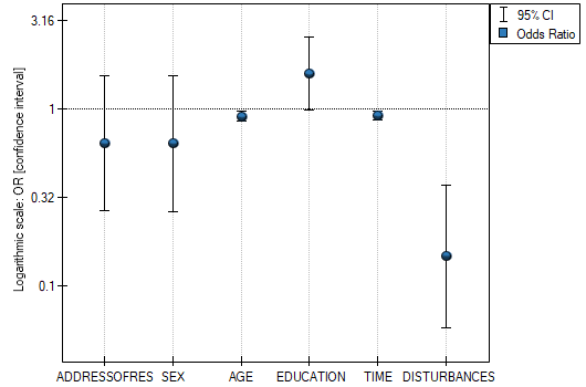
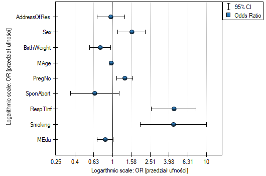
Odds Ratio with confidence interval – is a graph showing the OR along with the 95 percent confidence interval for the score of each variable returned in the constructed model. For categorical variables, the line at level 1 indicates the odds ratio value for the reference category.

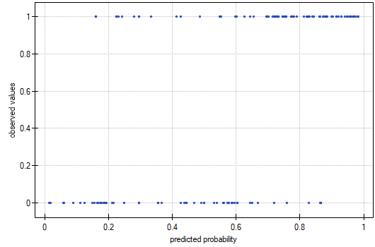
Observed Values / Expected Probability – is a graph showing the results of each person's predicted probability of an event occurring (X-axis) and the true value, which is the occurrence of the event (value 1 on the Y-axis) or the absence of the event (value 0 on the Y-axis). If the model predicts very well, points will accumulate at the bottom near the left side of the graph and at the top near the right side of the graph.

ROC curve – is a graph constructed based on the value of the dependent variable and the predicted probability of an event.

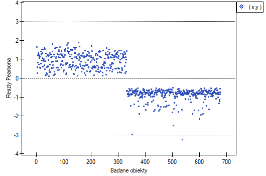
Pearson residuals plot – is a graph that allows you to assess whether there are outliers in the data. The residuals are the differences between the observed value and the probability predicted by the model. Plots of raw residuals from logistic regression are difficult to interpret, so they are unified by determining Pearson residuals. The Pearson residual is the raw residual divided by the square root of the variance function. The sign (positive or negative) indicates whether the observed value is higher or lower than the value fitted to the model, and the magnitude indicates the degree of deviation. Person's residuals less than or greater than 3 suggest that the variance of a given object is too largeu.

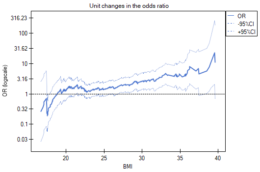
Unit changes in the odds ratio – is a graph showing a series of odds ratios, along with a confidence interval, determined for each possible cut-off point of a variable placed on the X axis. It allows the user to select one good cut-off point and then build from that a new bivariate variable at which a high or low odds ratio is achieved, respectively. The chart is dedicated to the evaluation of continuous variables in univariate analysis, i.e. when only one independent variable is selected.
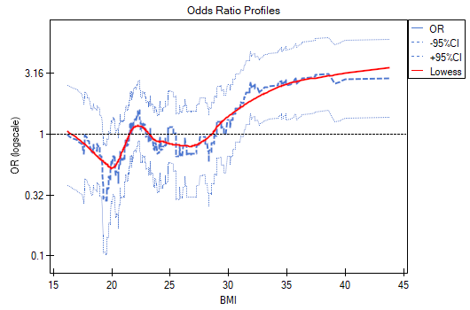
odds ratio profile is a graph presenting series of odds ratios with confidence interval, determined for a given window size, i.e. comparing frequencies inside the window with frequencies placed outside the window. It enables the user to choose several categories into which he wants to divide the examined variable and adopt the most advantageous reference category. It works best when we are looking for a U-shaped function i.e. high risk at low and at high values of the variable under study and low risk at average values. There is no one window size that is good for every analysis, the window size must be determined individually for each variable. The size of the window indicates the number of unique values of variable X contained in the window. The wider the window, the greater the generalizability of the results and the smoother the odds ratio function. The narrower the window, the more detailed the results, resulting in a more lopsided odds ratio function. A curve is added to the graph showing the smoothed (Lowess method) odds ratio value. Setting the smoothing factor close to 0 results in a curve closely fitting to the odds ratio, whereas setting the smoothing factor closer to 1 results in more generalized odds ratio, i.e. smoother and less fitting to the odds ratio curve. The graph is dedicated to the evaluation of continuous variables in univariate analysis, i.e. when only one independent variable is selected.

EXAMPLE (OR profiles.pqs file)

We examine the risk of disease A and disease B as a function of the patient's BMI. Since BMI is a continuous variable, its inclusion in the model results in a unit odds ratio that determines a linear trend of increasing or decreasing risk. We do not know whether a linear model will be a good model for the analysis of this risk, so before building multivariate logistic regression models, we will build some univariate models presenting this variable in graphs to be able to assess the shape of the relationship under study and, based on this, decide how we should prepare the variable for analysis. For this purpose, we will use plots of unit changes in odds ratio and odds ratio profiles, and for the profiles we will choose a window size of 100 because almost every patient has a different BMI, so about 100 patients will be in each window.

Disease A

Unit changes in the odds ratio show that when the BMI cut-off point is chosen somewhere between 27 and 37, we get a statistically significant and positive odds ratio showing that people with a BMI above this value have a significantly higher risk of disease than people below this value.

The odds ratio profiles show that the red curve is still close to 1, only the top of the curve is slightly higher, indicating that it may be difficult to divide BMI into more than 2 categories and select a good reference category, i.e., one that yields significant odds ratios.

In summary, one can use a split of BMI into two values (e.g., relate those with a BMI above 30 to those with a BMI below that, in which case OR[95%CI]=[1.41, 4.90], p=0.0024) or stay with the unit odds ratio, indicating a constant increase in disease risk with an increase in BMI of one unit (OR[95%CI]=1.07[1.02, 1.13], p=0.0052).

Disease B

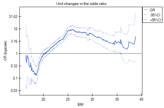
Unit changes in the odds ratio show that when the BMI cut-off point is chosen somewhere between 22 and 35, we get a statistically significant and positive odds ratio showing that people with a BMI above this value have a significantly higher risk of disease than those below this value.

The odds ratio profiles show that it would be much better to divide BMI into 2 or 4 categories. With the reference category being the one that includes a BMI somewhere between 19 and 25, as this is the category that is lowest and is far removed from the results for BMIs to the left and right of this range. We see a distinct U-like shape, meaning that disease risk is high at low BMI and at high BMI.

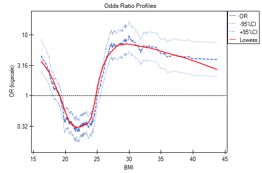
In summary, although the relationship for the unit odds ratio, or linear relationship, is statistically significant, it is not worth building such a model. It is much better to divide BMI into categories. The division that best shows the shape of this relationship is the one using two or three BMI categories, where the reference value will be the average BMI. Using the standard division of BMI and establishing a reference category of BMI in the normal range will result in a more than 15 times higher risk for underweight people (OR[95%CI]=15.14[6.93, 33.10]) more than 10 times for overweight people (OR[95%CI]=10.35[6.74, 15.90]) and more than twelve times for people with obesity (OR[95%CI]=12.22[6.94, 21.49]).

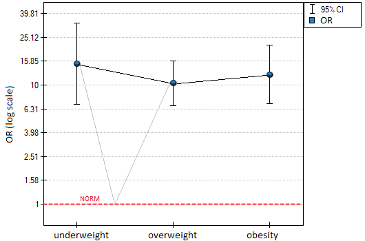
In the odds ratio plot, the BMI norm is indicated at level 1, as the reference category. We have drawn lines connecting the obtained ORs and also the norm, so as to show that the obtained shape of the relationship is the same as that determined previously by the odds ratio profile.

2022/02/09 12:56

Examples for logistic regression

EXAMPLE (anomaly.pqs file)

Studies have been conducted for the purpose of identifying the risk factors for a certain rare congenital anomaly in children. 395 mothers of children with that anomaly and 375 of healthy children have participated in that study. The gathered data are: address of residence, child's sex, child's weight at birth, mother's age, number of pregnancy, previous spontaneous abortions, respiratory tract infections, smoking, mother's education.

We construct a logistic regression model to check which variables may have a significant influence on the occurrence of the anomaly. The dependent variable is the column GROUP, the distinguished values in that variable as $1$ are the cases, that are mothers of children with anomaly. The following $9$ variables are independent variables:

AddressOfRes (2=city/1=village),

Sex (1=male/0=female),

BirthWeight (in kilograms, with an accuracy of 0.5 kg),

MAge (in years),

PregNo (which pregnancy is the child from),

SponAbort (1=yes/0=no),

RespTInf (1=yes/0=no),

Smoking (1=yes/0=no),

MEdu (1=primary or lower/2=vocational/3=secondary/4=tertiary).

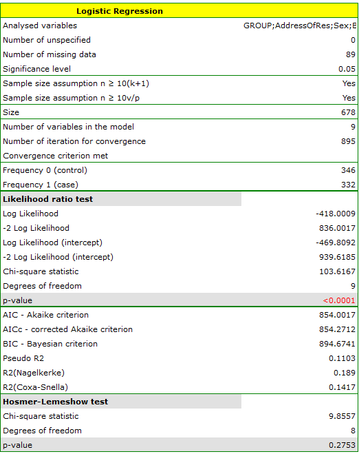
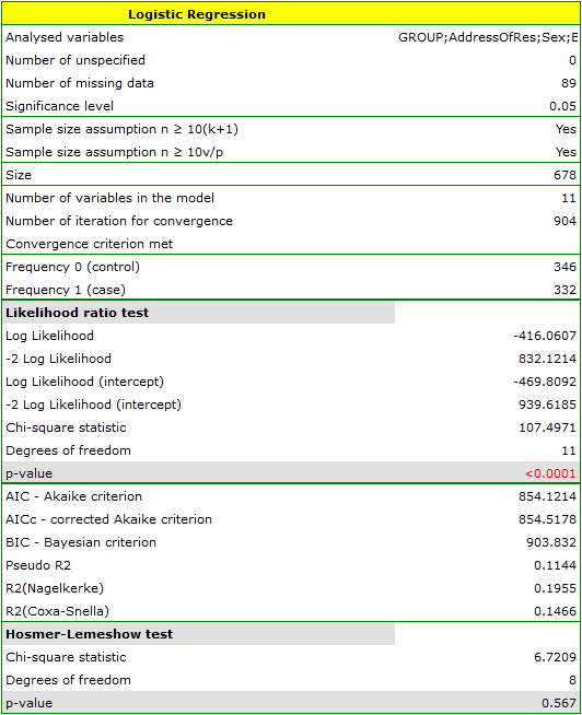
The quality of model goodness of fit is not high ( $R^2_{Pseudo}=0.11$ , $R^2_{Nagelkerke}=0.19$ i $R^2_{Cox-Snell}=0.14$ ). At the same time the model is statistically significant (value $p<0.000001$ of the Likelihood Ratio test), which means that a part of the independent variables in the model is statistically significant. The result of the Hosmer-Lemeshow test points to a lack of significance ( $p=0.2753$ ). However, in the case of the Hosmer-Lemeshow test we ought to remember that a lack of significance is desired as it indicates a similarity of the observed sizes and of predicted probability.

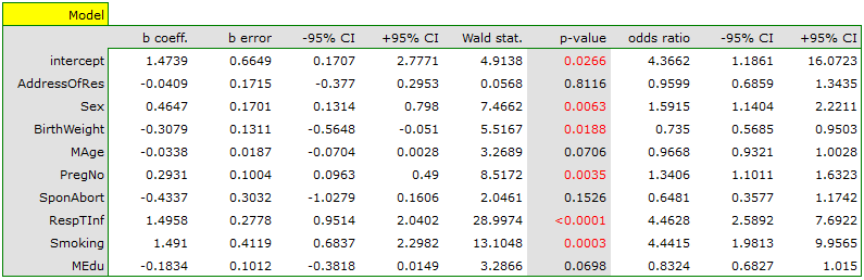
An interpretation of particular variables in the model starts from checking their significance. In this case the variables which are significantly related to the occurrence of the anomaly are:

Sex: $p=0.0063$ ,

BirthWeight: $p=0.0188$ ,

PregNo: $p=0.0035$ ,

RespTInf: $p<0.000001$ ,

Smoking: $p=0.0003$ .

The studied congenital anomaly is a rare anomaly but the odds of its occurrence depend on the variables listed above in the manner described by the odds ratio:

variable Sex: $OR[95%CI]=1.60[1.14;2.22]$ \textendash the odds of the occurrence of the anomaly in a boy is $1.6$ times greater than in a girl;
variable BirthWeight: $OR[95%CI]=0.74[0.57;0.95]$ \textendash the higher the birth weight the smaller the odds of the occurrence of the anomaly in a child;
variable PregNo: $OR[95%CI]=1.34[1.10;1.63]$ \textendash the odds of the occurrence of the anomaly in a child is $1.34$ times greater with each subsequent pregnancy;
variable RespTInf: $OR[95%CI]=4.46[2.59;7.69]$ \textendash the odds of the occurrence of the anomaly in a child if the mother had a respiratory tract infection during the pregnancy is $4.46$ times greater than in a mother who did not have such an infection during the pregnancy;
variable Smoking: $OR[95%CI]=4.44[1.98;9.96]$ \textendash a mother who smokes when pregnant increases the risk of the occurrence of the anomaly in her child $4.44$ times.

In the case of statistically insignificant variables the confidence interval for the Odds Ratio contains 1 which means that the variables neither increase nor decrease the odds of the occurrence of the studied anomaly. Therefore, we cannot interpret the obtained ratio in a manner similar to the case of statistically significant variables.

The influence of particular independent variables on the occurrence of the anomaly can also be described with the help of a chart concerning the odds ratio:

EXAMPLE continued (anomaly.pqs file)

Let us once more construct a logistic regression model, however, this time let us divide the variable mother's education into dummy variables (with dummy coding). With this operation we lose the information about the ordering of the category of education but we gain the possibility of a more in-depth analysis of particular categories. The breakdown into dummy variables is done by selecting Dummy var. in the analysis window.:

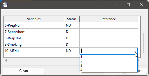
The primary education variable is missing as it will constitute the reference category.

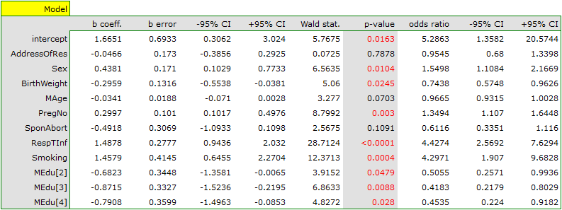
As a result the variables which describe education become statistically significant. The goodness of fit of the model does not change much but the manner of interpretation of the the odds ratio for education does change:

$\begin{tabular}{|l|l|} \hline \textbf{Variable}& $OR[95\%CI]$ \\\hline Primary education& reference category\\ Vocational education& $0.51[0.26;0.99]$\\ Secondary education& $0.42[0.22;0.80]$\\ Tertiary education& $0.45[0.22;0.92]$\\\hline \end{tabular}$

The odds of the occurrence of the studied anomaly in each education category is always compared with the odds of the occurrence of the anomaly in the case of primary education. We can see that for more educated the mother, the odds is lower. For a mother with:

vocational education the odds of the occurrence of the anomaly in a child is 0.51 of the odds for a mother with primary education;
secondary education the odds of the occurrence of the anomaly in a child is 0.42 of the odds for a mother with primary education;
tertiary education the odds of the occurrence of the anomaly in a child is 0.45 of the odds for a mother with primary education;

EXAMPLE (task.pqs file)

An experiment has been made with the purpose of studying the ability to concentrate of a group of adults in an uncomfortable situation. 190 people have taken part in the experiment (130 people are the teaching set, 40 people are the test set). Each person was assigned a certain task the completion of which requried concentration. During the experiment some people were subject to a disturbing agent in the form of temperature increase to 32 degrees Celsius. The participants were also asked about their address of residence, sex, age, and education. The time for the completion of the task was limited to 45 minutes. In the case of participants who completed the task before the deadline, the actual time devoted to the completion of the task was recorded. We will perform all our calculations only for those belonging to the teaching set. }

Variable SOLUTION (yes/no) contains the result of the experiment, i.e. the information about whether the task was solved correctly or not. The remaining variables which could have influenced the result of the experiment are:

ADDRESSOFRES (1=city/0=village),

SEX (1=female/0=male),

AGE (in years),

EDUCATION (1=primary, 2=vocational, 3=secondary, 4=tertiary),

TIME needed for the completion of the task (in minutes),

DISTURBANCES (1=yes/0=no).

On the basis of all those variables a logistic regression model was built in which the distinguished state of the variable SOLUTION was set to „yes”.

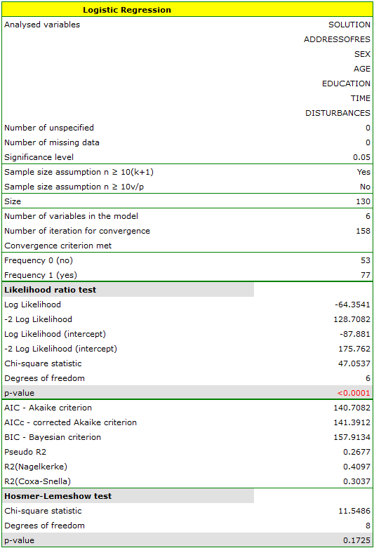
The adequacy quality is described by the coefficients: $R^2_{Pseudo}=0.27$ , $R^2_{Nagelkerke}=0.41$ i $R^2_{Cox-Snell}=0.30$ . The sufficient adequacy is also indicated by the result of the Hosmer-Lemeshow test $(p=0.1725)$ . The whole model is statistically significant, which is indicated by the result of the Likelihood Ratio test $(p<0.000001)$ .

The observed values and predicted probability can be observed on the chart:

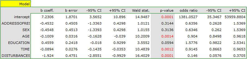
In the model the variables which have a significant influence on the result are:

AGE: p=0.0014,

TIME: p=0.0012,

DISTURBANCES: <p=0.0001.

What is more, the younger the person who solves the task the shorter the time needed for the completion of the task, and if there is no disturbing agent, the probability of correct solution is greater:

AGE: $OR[95%CI]=0.90[0.85;0.96]$ ,

TIME: $OR[95%CI]=0.91[0.87;0.97]$ ,

DISTURBANCES: $OR[95%CI]=0.15[0.06;0.37]$ .

The obtained results of the Odds Ratio are presented on the chart below:

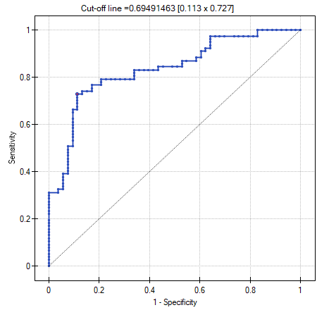
Should the model be used for prediction, one should pay attention to the quality of classification. For that purpose we calculate the ROC curves.

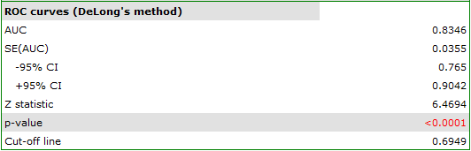
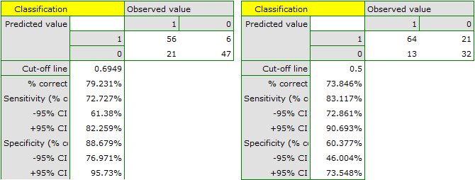
The result seems satisfactory. The area under the curve is $AUC=0.83$ and is statistically greater than $0.5$ $(p<0.0001)$ , so classification is possible on the basis of the constructed model. The suggested cut-off point for the ROC curve is $0.6949$ and is slightly higher than the standard level used in regression, i.e. $0.5$ . The classification determined from this cut-off point yields $79.23%$ of cases classified correctly, of which correctly classified yes values are $72.73%$ (sensitivity), no values are $88.68%$ (specificity). The classification derived from the standard value yields no less, $73.85%$ of cases classified correctly, but it will yield more correctly classified yes values are $83.12%$ , although less correctly classified no values are $60.38\%$ .

We can finish the analysis of classification at this stage or, if the result is not satisfactory, we can make a more detailed analysis of the ROC curve in module ROC curve.

As we have assumed that classification on the basis of that model is satisfactory we can calculate the predicted value of a dependent variable for any conditions. Let us check what odds of solving the task has a person whose:

ADDRESSOFRES (1=city),

SEX (1=female),

AGE (50 years),

EDUCATION (1=primary),

TIME needed for the completion of the task (20 minutes),

DISTURBANCES (1=yes).

For that purpose, on the basis of the value of coefficient $b$ , we calculate the predicted probability (probability of receiving the answer „yes” on condition of defining the values of dependent variables):

$\begin{displaymath} \begin{array}{l} P(Y=yes|ADDRESSOFRES,SEX,AGE,EDUCATION,TIME,DISTURBANCES)=\\[0.2cm] =\frac{e^{7.23-0.45\textrm{\scriptsize \textit{ADDRESSOFRES}}-0.45\textrm{\scriptsize\textit{SEX}}-0.1\textrm{\scriptsize\textit{AGE}}+0.46\textrm{\scriptsize\textit{EDUCATION}}-0.09\textrm{\scriptsize\textit{TIME}}-1.92\textrm{\scriptsize\textit{DISTURBANCES}}}}{1+e^{7.23-0.45\textrm{\scriptsize\textit{ADDRESSOFRES}}-0.45\textrm{\scriptsize\textit{SEX}}-0.1\textrm{\scriptsize\textit{AGE}}+0.46\textrm{\scriptsize\textit{EDUCATION}}-0.09\textrm{\scriptsize\textit{TIME}}-1.92\textrm{\scriptsize\textit{DISTURBANCES}}}}=\\[0.2cm] =\frac{e^{7.231-0.453\cdot1-0.455\cdot1-0.101\cdot50+0.456\cdot1-0.089\cdot20-1.924\cdot1}}{1+e^{7.231-0.453\cdot1-0.455\cdot1-0.101\cdot50+0.456\cdot1-0.089\cdot20-1.924\cdot1}} \end{array} \end{displaymath}$

As a result of the calculation the program will return the result:

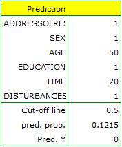
The obtained probability of solving the task is equal to $0.1215$ , so, on the basis of the cut-off $0.60$ , the predicted result is $0$ \textendash which means the task was not solved correctly.

2022/02/09 12:56

Model-based prediction and test set validation

Validation

Validation of a model is a check of its quality. It is first performed on the data on which the model was built (the so-called training data set), that is, it is returned in a report describing the resulting model. To be able to judge with greater certainty how suitable the model is for forecasting new data, an important part of the validation is to apply the model to data that were not used in the model estimation. If the summary based on the training data is satisfactory, i.e. the determined errors, $R^2$ coefficients and information criteria are at a satisfactory level, and the summary based on the new data (the so-called test data set) is equally favorable, then with high probability it can be concluded that such a model is suitable for prediction. The test data should come from the same population from which the training data were selected. It is often the case that before building a model we collect data, and then randomly divide it into a training set, i.e. the data that will be used to build the model, and a test set, i.e. the data that will be used for additional validation of the model.
The settings window with the validation can be opened in Advanced statistics→Multivariate models→Logistic regression - prediction/validation.

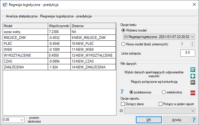
To perform validation, it is necessary to indicate the model on the basis of which we want to perform the validation. Validation can be done on the basis of:

logistic regression model built in PQStat - simply select a model from the models assigned to the sheet, and the number of variables and model coefficients will be set automatically; the test set should be in the same sheet as the training set;
model not built in PQStat but obtained from another source (e.g., described in a scientific paper we have read) - in the analysis window, enter the number of variables and enter the coefficients for each of them.

In the analysis window, indicate those new variables that should be used for validation.

Prediction

Most often, the final step in regression analysis is to use the built and previously validated model for prediction.

Prediction for a single object can be performed along with model building, that is, in the analysis window Advanced statistics→Multivariate models→Logistic regression ,
Predykcja dla większej grupy nowych danych jest wykonywana poprzez menuAdvanced statistics→Multivariate models→Logistic regression - prediction/validation.

To make a prediction, it is necessary to indicate the model on the basis of which we want to make the prediction. Prediction can be made on the basis of:

logistic regression model built in PQStat - simply select a model from the models assigned to the sheet, and the number of variables and model coefficients will be set automatically; the test set should be in the same sheet as the training set;
model not built in PQStat but obtained from another source (e.g., described in a scientific paper we have read) - in the analysis window, enter the number of variables and enter the coefficients for each of them.

In the analysis window, indicate those new variables that should be used for prediction. Based on the new data, the value of the probability predicted by the model is determined and then the prediction of the occurrence of an event (1) or its absence (0). The cutoff point based on which the classification is performed is the default value $0.5$ . The user can change this value to any value in the range $(0-1)$ such as the value suggested by the ROC curve.

Przykład c.d. (task.pqs file)

In an experiment examining concentration skills, a logistic regression model was built for a group of 130 training set subjects based on the following variables:

dependent variable: SOLUTION (yes/no) - information about whether the task was solved correctly or not;

independent variables:

ADDRESSOFRES (1=urban/0=rural),

SEX (1=female/0=male),

AGE (in years),

EDUCATION (1=basic, 2=vocational, 3=secondary, 4=higher education),

SOLUTION Time (in minutes),

DISTURBANCES (1=yes/0=no).

However, only four variables, AGE, EDUCATION, RESOLUTION TIME, and DISTURBANCES, contribute relevant information to the model. We will build a model for the training set data based on these four variables and then, to make sure it will work properly, we will validate it on a test data set. If the model passes this test, we will use it to make predictions for new individuals. To use the right collections we set a data filter each time.

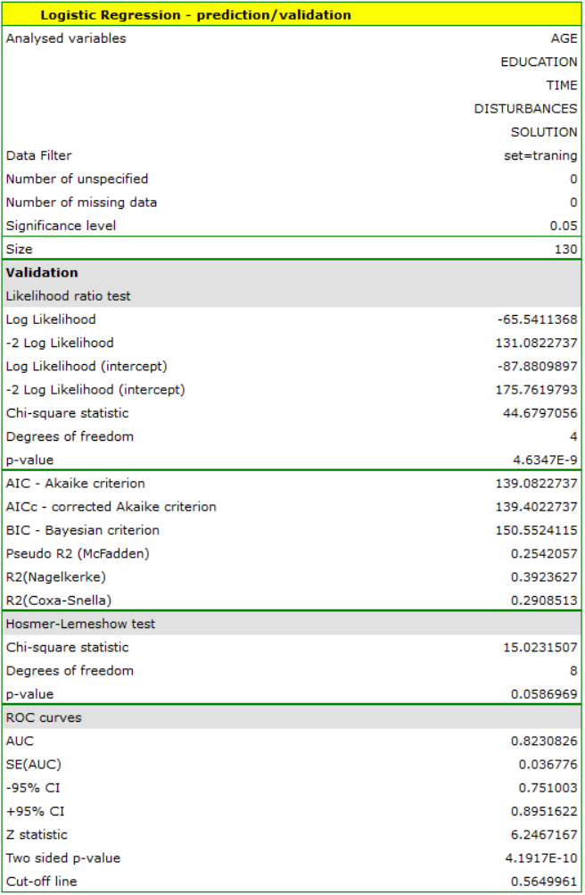
For the training set, the values describing the quality of the model's fit are not very high $Pseudo R^2 = 0.26$ and $R^2(Nagelkerke) = 0.39$ , but already the quality of its prediction is satisfactory (AUC[95%CI]=0.82[0.75, 0.90], sensitivity =82%, specificity 60%).

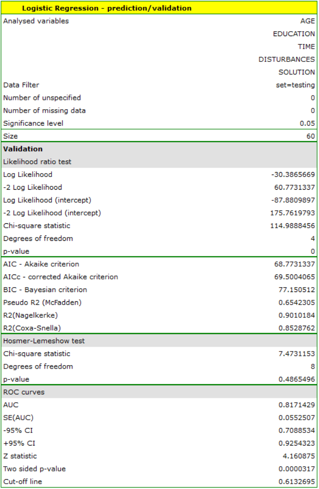
For the test set, the values describing the quality of the model fit are even higher than for the training data $Pseudo R^2 = 0.65$ and $R^2(Nagelkerke) = 0.90$ . The prediction quality for the test data is still satisfactory (AUC[95%CI]=0.82[0.71, 0.93], sensitivity =73%, specificity 64%), so we will use the model for prediction. To do this, we will use the data of three new individuals added at the end of the set. We'll select Prediction, set a filter on the new dataset, and use our model to predict whether the person will solve the task correctly (get a value of 1) or incorrectly (get a value of 0).

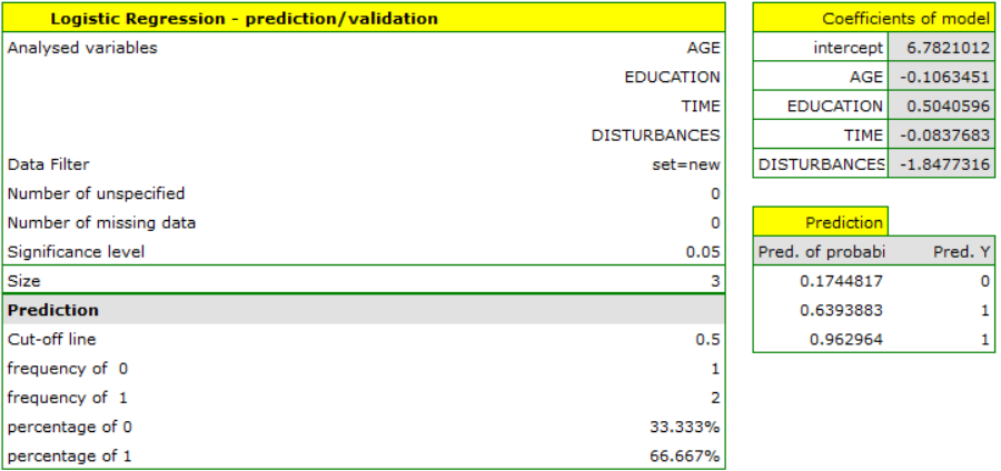
We find that the prediction for the first person is negative, while the prediction for the next two is positive. The prognosis for a 50-year-old woman with an elementary education solving the test during the interference in 20 minutes is 0.17, which means that we predict that she will solve the task incorrectly, while the prognosis for a woman 20 years younger is already favorable - the probability of her solving the task is 0.64. The highest probability (equal to 0.96) of a correct solution has the third woman, who solved the test in 10 minutes and without disturbances.

If we wanted to make a prediction based on another model (e.g., obtained during another scientific study: SOLUTION=6-0.1*AGE+0.5*EDUCATION-0.1*TIME-2*DISTURBANCES) - it would be enough to select a new model in the analysis window, set its coefficients and the forecast for the selected people can be repeated based on this model.

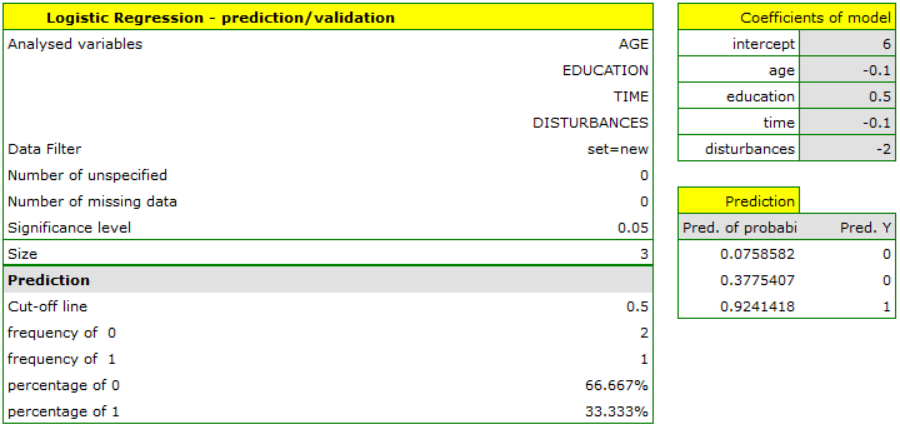
This time, according to the prediction of the new model, the prediction for the first and second person is negative, and the third is positive.

2022/02/09 12:56

¹⁾

Peduzzi P., Concato J., Kemper E., Holford T.R., Feinstein A.R. (1996), A simulation study of the number of events per variable in logistic regression analysis. J Clin Epidemiol;49(12):1373-9

PQStat - Baza Wiedzy

Narzędzia użytkownika

Narzędzia witryny

Pasek boczny

Spis treści

Logistic regression

The Odds Ratio

Model verification

Graphs in logistic regression

Examples for logistic regression

Model-based prediction and test set validation

Narzędzia strony