Analyses for contingency tables

Analyses for the contingency tables can be computed from data collected in the contingency tables or directly i.e., from raw data. Whereby it is possible to transform the data from the contingency table to the raw form or vice versa.

EXAMPLE (sex-education.pqs file)

Consider a sample consisting of 34 individuals ( $n=34$ ). We examine 2 traits of these individuals ( $X$ =sex, $Y$ =education). Gender appears in 2 categories ( $X_1$ =female, $X_2$ =male) education in 3 categories, ( $Y_1$ =primary + vocational $Y_2$ =medium, $Y_3$ =higher).

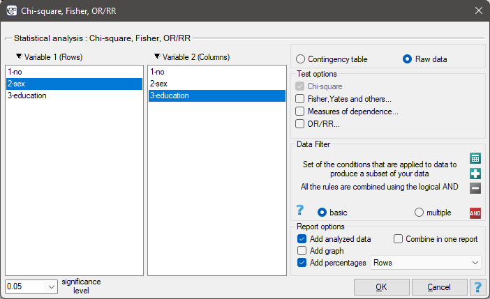
In the case of raw data, when you open the test options window, e.g., the $\chi^2$ for the $C\times R$ tables, the raw data option will automatically be selected..

For data collected in a contingency table, it is a good idea to select this data (numerical values without headers) before opening the test window. Then, when you open the test window, the contingency table option will automatically be selected and the data from the selection will be displayed.

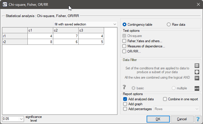
In the test window, we can always change the automatically detected setting regarding the form of data organization, as well as enter data into the contingency table from the window.

Cochran's condition

This is a basic condition for using many statistical tests based on contingency tables, e.g., the chi-square test. This condition implies a large expectred frequencies. According to Cochran's 1952 interpretation¹⁾, none of the expected frequencies can be $<1$ and no more than 20% can be $<5$ . Information about whether this condition is met (or not) by the data collected in the table can be returned to the report.

Basic tests for contingency tables:

Coefficients for contingency tables:

You can also include a basic summary of the tables in the results report:

Contingency table of observed frequencies $-$ that is, data in the form of a contingency table. Such a table shows the distribution of observations for several traits (several variables). Table for 2 traits ( $X$ , $Y$ ), of which the first has possible $r$ and the second $c$ categories are shown below).

$\begin{tabular}{|c|c||c|c|c|c|c|} \hline \multicolumn{2}{|c||}{Frequencies}& \multicolumn{5}{|c|}{Trait Y}\\\cline{3-7} \multicolumn{2}{|c||}{ observed $O_{ij}$} & $Y_1$ & $Y_2$ & ... & $Y_c$ & Total \\\hline \hline \multirow{5}{*}{Trait $X$}& $X_1$ & $O_{11}$ & $O_{12}$ & ... & $O_{1c}$& $\sum_{j=1}^cO_{1j}$ \\\cline{2-7} & $X_2$ & $O_{21}$ & $O_{22}$ & ... & $O_{2c}$& $\sum_{j=1}^cO_{2j}$ \\\cline{2-7} & ...& ... & ... & ... & ...& ... \\\cline{2-7} & $X_r$ & $O_{r1}$ & $O_{r2}$ & ... & $O_{rc}$& $\sum_{j=1}^cO_{rj}$ \\\cline{2-7} & Suma & $\sum_{i=1}^rO_{i1}$ & $\sum_{i=1}^rO_{i2}$ & ... & $\sum_{i=1}^rO_{ic}$& $n=\sum_{i=1}^r\sum_{j=1}^cO_{ij}$\\\hline \end{tabular}$

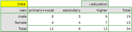
Frequencies observed $O_{ij}$ ( $i=1,2,\dots,r;j=1,2,\dots,c$ ) represent the frequency of each category for both traits.

In order for such a table to be returned by the program, the option include analysed data should be selected in the test window. For the data from the example, the contingency table of observed frequencies is as follows:

A contingency table of expected frequencies $-$ for each contingency table of observed frequencies, a corresponding table of expected frequencies: $E_{ij}$ can be created

$\begin{tabular}{|c|c||c|c|c|c|} \hline \multicolumn{2}{|c||}{frequencies }& \multicolumn{4}{|c|}{Trait Y}\\\cline{3-6} \multicolumn{2}{|c||}{expected $E_{ij}$} & $Y_1$ & $Y_2$ & ... & $Y_c$ \\\hline \hline \multirow{4}{*}{Trait $X$}& $X_1$ & $E_{11}$ & $E_{12}$ & ... & $E_{1c}$\\\cline{2-6} & $X_2$ & $E_{21}$ & $E_{22}$ & ... & $E_{2c}$ \\\cline{2-6} & ...& ... & ... & ... & ... \\\cline{2-6} & $X_r$ & $E_{r1}$ & $E_{r2}$ & ... & $E_{rc}$\\\hline \end{tabular}$

where:

$E_{11}=\frac{\sum_{i=1}^rO_{i1}\times\sum_{j=1}^cO_{1j}}{n}$ , $E_{12}=\frac{\sum_{i=1}^rO_{i2}\times\sum_{j=1}^cO_{1j}}{n}$ , $E_{1c}=\frac{\sum_{i=1}^rO_{ic}\times\sum_{j=1}^cO_{1j}}{n}$

$E_{21}=\frac{\sum_{i=1}^rO_{i1}\times\sum_{j=1}^cO_{2j}}{n}$ , $E_{22}=\frac{\sum_{i=1}^rO_{i2}\times\sum_{j=1}^cO_{2j}}{n}$ , $E_{2c}=\frac{\sum_{i=1}^rO_{ic}\times\sum_{j=1}^cO_{2j}}{n}$

$E_{r1}=\frac{\sum_{i=1}^rO_{i1}\times\sum_{j=1}^cO_{rj}}{n}$ , $E_{r2}=\frac{\sum_{i=1}^rO_{i2}\times\sum_{j=1}^cO_{rj}}{n}$ , $E_{rc}=\frac{\sum_{i=1}^rO_{ic}\times\sum_{j=1}^cO_{rj}}{n}$ .

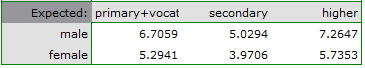
For the data in the example The contingency table of expected frequencies is as follows:

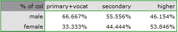
Contingency table of percentages calculated from the sum of columns. For the data in the example this table is as follows:

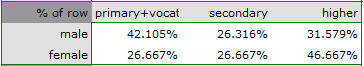
Tcontingency table of percentages calculated from the sum of the rows. For the data in the example this table is as follows:

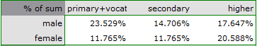
A contingency table of percentages calculated from the sum of the total rows and columns. For the data in the example this table is as follows:

¹⁾

Cochran W.G. (1952), The chi-square goodness-of-fit test. Annals of Mathematical Statistics, 23, 315-345

PQStat - Baza Wiedzy

Pasek boczny

Analyses for contingency tables

PQStat - Baza Wiedzy

Narzędzia użytkownika

Narzędzia witryny

Pasek boczny

Analyses for contingency tables

Narzędzia strony