PQStat - Baza Wiedzy

The Chi-square test for trend

The $\chi^2$ test for trend (also called the Cochran-Armitage trend test ¹⁾²⁾)is used to determine whether there is a trend in proportion for particular categories of an analysed variables (features). It is based on the data gathered in the contingency tables of 2 features. The first feature has the possible $r$ ordered categories: $X_1, X_2,..., X_r$ and the second one has 2 categories: $G_1$ , $G_2$ . The contingency table of $r\times 2$ observed frequencies

$\begin{tabular}{|c|c||c|c|c|} \hline \multicolumn{2}{|c||}{Observed frequencies }& \multicolumn{3}{|c|}{Feature 2 (group)}\\\cline{3-5} \multicolumn{2}{|c||}{$O_{ij}$} & $G_1$ & $G_2$ & Total \\\hline \hline \multirow{5}{*}{Feature 1 (feature $X$)}& $X_1$& $O_{11}$ & $O_{12}$ & $W_1=O_{11}+O_{12}$ \\\cline{2-5} & $X_2$ & $O_{21}$ & $O_{22}$ & $W_2=O_{21}+O_{22}$ \\\cline{2-5} & ... & ... & ... & ... \\\cline{2-5} & $X_r$ & $O_{r1}$ & $O_{r2}$ & $W_r=O_{r1}+O_{r2}$ \\\cline{2-5} & Total & $C_1=\sum_{i=1}^rO_{i1}$ & $C_2=\sum_{i=1}^rO_{i2}$ & $n=C_1+C_2$\\\hline \end{tabular}$

Basic assumptions:

measurement on an ordinal scale or on an interval scale,
an independent model (the second feature - 2 independent groups).

Hypotheses:

$\begin{array}{cl} \mathcal{H}_0: & $In the analysed population the trend in a proportion of $p_1, p_2, ..., p_r$ does not exist, $\\ \mathcal{H}_1: & $There is the trend in a proportion of $p_1, p_2, ..., p_r$ in the analysed population. $ \end{array}$

where:

$p_1, p_2, ..., p_r$ are the proportions $p_1=\frac{O_{11}}{W_1}$ , $p_2=\frac{O_{21}}{W_2}$ ,…, $p_r=\frac{O_{r1}}{W_r}$ .

The test statistic is defined by:

$\begin{displaymath} \chi^2=\frac{\left[\left(\sum_{i=1}^r i\cdot O_{i1}\right) -C_1\left(\sum_{i=1}^r\frac{i\cdot W_i}{n}\right)\right]^2}{\frac{C_1}{n}\left(1-\frac{C_1}{n}\right)\left[\left(\sum_{i=1}^n i^2 W_i\right)-n\left(\sum_{i=1}^n\frac{i \cdot W_i}{n}\right)^2\right]}. \end{displaymath}$

This statistic asymptotically (for large expected frequencies) has the Chi-square distribution with 1 degree of freedom.

The p-value, designated on the basis of the test statistic, is compared with the significance level $\alpha$ :

$\begin{array}{ccl} $ if $ p \le \alpha & \Longrightarrow & $ reject $ \mathcal{H}_0 $ and accept $ \mathcal{H}_1, \\ $ if $ p > \alpha & \Longrightarrow & $ there is no reason to reject $ \mathcal{H}_0. \\ \end{array}$

The settings window with the Chi-square test for trend can be opened in Statistics menu → NonParametric tests → Chi-square, Fisher, OR/RR → Chi-square for trend.

EXAMPLE (smoking-education.pqs file)

We examine whether cigarette smoking is related to the education of residents of a village. A sample of 122 people was drawn. The data were recorded in a file. }

We assume that the relationship can be of two types i.e. the more educated people, the more often they smoke or the more educated people, the less often they smoke. Thus, we are looking for an increasing or decreasing trend.

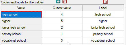
Before proceeding with the analysis, we need to prepare the data, i.e., we need to indicate the order in which the education categories should appear. To do this, from the properties of the Education variable, we select Codes/Labels/Format… and assign the order by specifying consecutive natural numbers. We also assign labels.

Hypotheses:

$\begin{array}{cl} \mathcal{H}_0: & $there is no trend in the rural population of increasing/decreasing $\\ & $wraz ze wzrostem wykształcenia, $\\ \mathcal{H}_1: & $there is a trend in the rural population of increasing/decreasing $\\ & $numbers of smokers with increasing education. $ \end{array}$

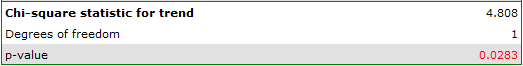
A p-value=0.0091, which compared to a significance level of $\alpha$ =0.05 indicates that the alternative hypothesis that a trend exists is true.

As the graph shows, the more educated people are, the less often they smoke. However, the result obtained by people with junior high school education deviates from this trend. Since there are only two people with lower secondary school education, it did not have much influence on the trend. Due to the very small size of this group, it was decided to repeat the analysis for the combined primary and lower secondary education categories.

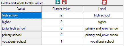
A small value was again obtained p=0.0078 and confirmation of a statistically significant trend.

EXAMPLE(viewers.pqs file)

Because of the decrease in people watching some particular soap opera there was carried out an opinion survey. 100 persons were asked, who has recently started watching this soap opera, and 300 persons were asked, who has watched it regularly from the beginning. They were asked about the level of preoccupation with the character's life. The results are written down in the table below:

$\begin{tabular}{|c||c|c|c|} \hline Level of & \multicolumn{3}{|c|}{group}\\\cline{2-4} commitment & group of new viewers & group of steady viewers & total \\\hline \hline rather small & 7 & 7 & 14 \\\hline average & 13 & 25 & 38 \\\hline rather high & 30 & 58 & 88 \\\hline high& 24 & 99 & 123\\\hline very high & 26& 111& 137\\\hline total & 100 & 300& 400\\\hline \end{tabular}$

The new viewers consist of 25\% of all the analysed viewers. This proportion is not the same for each level of commitment, but looks like this:

$\begin{tabular}{|c||c|c|c|} \hline Level of& \multicolumn{3}{|c|}{group}\\\cline{2-4} commitment & group of new viewers & group of steady viewers & total \\\hline \hline rather small & $p_1$=50.00\% & 50.00\% & 100\% \\\hline average & $p_2$=34.21\% & 65.79\% & 100\% \\\hline rather high & $p_3$=34.09\% & 65.91\% & 100\% \\\hline high& $p_4$=19.51\% & 80.49\% & 100\%\\\hline very high & $p_5$=18.98\%& 81.02\%& 100\%\\\hline \textbf{total} & \textbf{25.00\%} & \textbf{75.00\%}& \textbf{100\%}\\\hline \end{tabular}$

Hypotheses:

$\begin{array}{cl} \mathcal{H}_0: & $in the population of the soap opera viewers, the trend in proportions of $\\ & p_1, p_2, p_3, p_4, p_5 $ does not exist,$\\ \mathcal{H}_1: & $in the population of the soap opera viewers, the trend in proportions of $\\ & p_1, p_2, p_3, p_4, p_5 $ does exists.$\\ \end{array}$

The p-value=0.0004 which, compared to the significance level $\alpha$ =0.05, proves the truth of the alternative hypothesis that there is a trend in the proportions $p_1, p_2, ..., p_5$ . As can be seen from the contingency table of the percentages calculated from the sum of the columns, this is a decreasing trend (the more interested the group of viewers is in the fate of the characters of the series, the smaller part of it is made up of new viewers).

¹⁾

Cochran W.G. (1954), Some methods for strengthening the common chi-squared tests. Biometrics. 10 (4): 417–451

²⁾

Armitage P. (1955), Tests for Linear Trends in Proportions and Frequencies. Biometrics. 11 (3): 375–386

PQStat - Baza Wiedzy

Narzędzia użytkownika

Narzędzia witryny

Pasek boczny

The Chi-square test for trend

Narzędzia strony