Narzędzia użytkownika
Narzędzia witryny
Pasek boczny
en:statpqpl:porown2grpl:nparpl
Spis treści
Non-parametric tests
The Mann-Whitney U test
The Mann-Whitney  test is also called as the Wilcoxon Mann-Whitney test (Mann and Whitney (1947)1) and Wilcoxon (1949)2)). This test is used to verify the hypothesis that there is no shift in the compared distributions, i.e., most often the insignificance of differences between medians of an analysed variable in 2 populations (but you should assume that the distributions of a variable are pretty similar to each other - comparison of rank variances can be performed with the Conover rank test.
Basic assumptions:
- measurement on an ordinal scale or on an interval scale,
Hypotheses:

where:
 distributions of an analysed variable of the 1st and the 2nd population.
The p-value, designated on the basis of the test statistic, is compared with the significance level  :
:

Note
Depending on a sample size, the test statistic is calculated using by different formulas:
- For a small sample size:

or

where  are sample sizes,
  are rank sums for the samples.
This statistic has the Mann-Whitney distribution and it does not contain any correction for ties. The value of the exact probability of the Mann-Whitney distribution is calculated with the accuracy up to the hundredth place of the fraction.
- For a large sample size:

 ,
,
 – number of cases included in a
The formula for the  statistic includes the correction for ties. This correction is used, when ties occur (if there are no ties, the correction is not calculated, because of
  )
)
The statistic asymptotically (for large sample sizes) has the normal distribution.
The Mann-Whitney test with the continuity correction (Marascuilo and McSweeney (1977)3))
The continuity correction should be used to guarantee the possibility of taking in all the values of real numbers by the test statistic, according to the assumption of the normal distribution. The formula for the test statistic with the continuity correction is defined as:

Standardized effect size
The distribution of the Mann-Whitney test statistic is approximated by the normal distribution, which can be converted to an effect size  4) to then obtain the Cohen's d value according to the standard conversion used for meta-analyses:

When interpreting an effect, researchers often use general guidelines proposed by 5) defining small (0.2), medium (0.5) and large (0.8) effect sizes.
The settings window with the Mann-Whitney U test can be opened in Statistics menu → NonParametric tests (ordered categories) → Mann-Whitney or in ''Wizard''.
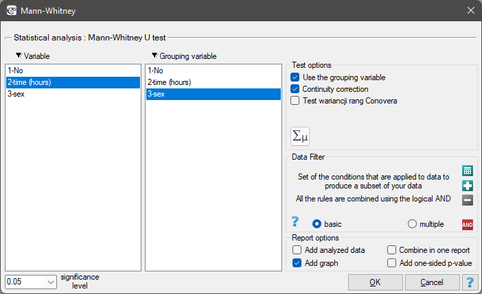
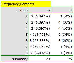
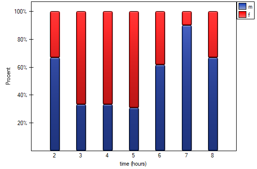
There was made a hypothesis that at some university male math students spend statistically more time in front of a computer screen than the female math students. To verify the hypothesis from the population of people who study math at this university, there was drawn a sample consisting of 54 people (25 women and 29 men). These persons were asked how many hours they spend in front of the computer screens daily. There were obtained the following results:
(time, sex): (2, k) (2, m) (2, m) (3, k) (3, k) (3, k) (3, k) (3, m) (3, m) (4, k) (4, k) (4, k) (4, k) (4, m) (4, m) (5, k) (5, k) (5, k) (5, k) (5, k) (5, k) (5, k) (5, k) (5, k) (5, m) (5, m) (5, m) (5, m) (6, k) (6, k) (6, k) (6, k) (6, k) (6, m) (6, m) (6, m) (6, m) (6, m) (6, m) (6, m) (6, m) (7, k) (7, m) (7, m) (7, m) (7, m) (7, m) (7, m) (7, m) (7, m) (7, m) (8, k) (8, m) (8, m).}
Hypotheses:

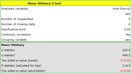
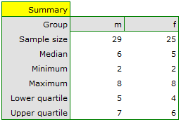
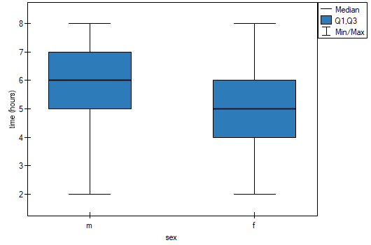
Based on the assumed  and the statistic of the Mann-Whitney test without correction for continuity (p=0.0154) as well as with this correction p=0.0158, as well as on the exact statistic (p=0.0149) we can assume that there are statistically significant differences between female and male math students in the amount of time spent in front of the computer. These differences are that female students spend less time in front of the computer than male students. They can be described by the median, quartiles, and the largest and smallest value, which we also see in a box-and-whisker plot. Another way to describe the differences is to represent the time spent in front of the computer based on a table of counts and percentages (which we run in the analysis window by setting descriptive statistics includegraphics
  ) or based on a column plot.
The Wilcoxon test (matched-pairs)
The Wilcoxon matched-pairs test, is also called as the Wilcoxon test for dependent groups (Wilcoxon 19456),19497)). It is used if the measurement of an analysed variable you do twice, each time in different conditions. It is the extension for the two dependent samples of the Wilcoxon test (signed-ranks) – designed for a one sample. We want to check how big is the difference between the pairs of measurements ( ) for each of
  analysed objects. This difference is used to verify the hypothesis determining that the median of the difference in the analysed population counts to 0.
Basic assumptions:
- measurement on an ordinal scale or on an interval scale,
Hypotheses:

where:
 – median of the differences
  in a population.
The p-value, designated on the basis of the test statistic, is compared with the significance level :
Note
Depending on the sample size, the test statistic is calculated by using different formulas:
- For small a sample size:

 – sums of positive
  – sums of negative ranks.
This statistic has the Wilcoxon distribution and does not contain any correction for ties.
- For a large sample size

The formula for the Z statistic includes the correction for ties. This correction is used, when the ties occur (if there are no ties, the correction is not calculated, because of  ).
).
The statistic (for large sample sizes) asymptotically has the normal distribution.
The Wilcoxon test with the continuity correction (Marascuilo and McSweeney (1977)8))
The continuity correction is used to guarantee the possibility of taking in all the values of the real numbers by the test statistic, according to the assumption of the normal distribution. The test statistic with the continuity correction is defined by:

Note
The median calculated for the difference column includes all pairs of results except those with a difference of 0.
Standardized effect size
The distribution of the Wilcoxon test statistic is approximated by the normal distribution, which can be converted to an effect size  9) to then obtain the Cohen's d value according to the standard conversion used for meta-analyses:
When interpreting an effect, researchers often use general guidelines proposed by 10) defining small (0.2), medium (0.5) and large (0.8) effect sizes.
The settings window with the Wilcoxon test for dependent groups can be opened in Statistics menu → NonParametric tests→Wilcoxon (matched-pairs) or in ''Wizard''.

There was chosen a sample consisting of 22 patients suffering from a cancer. They were examined to check the level of felt pain (1 – 10 scale, where 1 means the lack of pain and 10 means unbearable pain). This examination was repeated after a month of the treatment with a new medicine which was supposed to lower the level of felt pain. There were obtained the following results:
(pain before, pain after): (2, 2) (2, 3) (3, 1) (3,1) (3, 2) (3, 2) (3, 3) (4, 1) (4, 3) (4, 4) (5, 1) (5, 1) (5, 2) (5, 4) (5, 4) (6, 1) (6, 3) (7, 2) (7, 4) (7, 4) (8, 1) (8, 3). Now, you want to check if this treatment has any influence on the level of felt pain in the population, from which the sample was chosen.
Hypotheses:

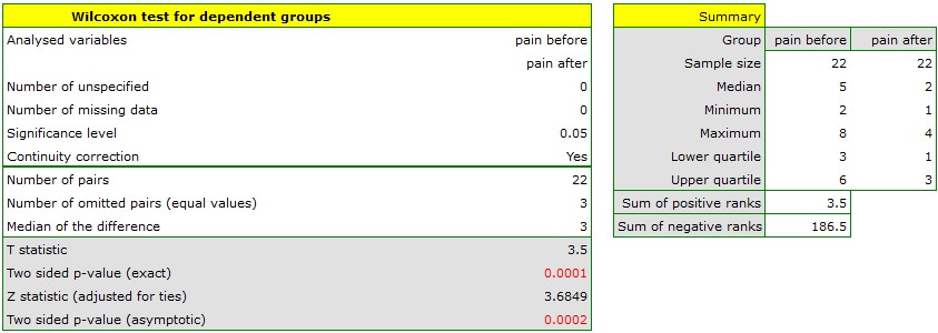
Comparing the  </latex> value = 0.0001 of the Wilcoxon test, based on the
  statistic, with the significance level you assume, that there is a statistically significant difference if concerning the level of felt pain between these 2 examinations. The difference is, that the level of pain decreased (the sum of the negative ranks is significantly greater than the sum of the positive ranks). Exactly the same decision you would make on the basis of
  value = 0.00021 or value = 0.00023 of the Wilcoxon test which is based on the statistic or the statistic with the continuity correction. We can see the differences in a box-and-whisker plot or a column plot.


The Chi-square tests
These tests are based on data collected in the form of a contingency table of 2 traits, trait X and trait Y, the former having  and the latter
  categories, so the resulting table has rows and columns. Therefore, we can speak of the 2×2 chi-square test (for tables with two rows and two columns) or the RxC chi-square test (with multiple rows and columns)).
We can read the details of the chi-square test of the two features here:
Basic assumptions:
- measurement on a nominal scale - any order is not taken into account,
The additional assumption for the  :
:
General hypotheses:

where:
 – observed frequencies in a contingency table,
 – expected frequencies in a contingency table.
Hypotheses in the meaning of independence:

The p-value, designated on the basis of the test statistic, is compared with the significance level :
Additionally
- In addition to the chi-square test, another related test may need to be determined. In the event that Cochran's condition is not satisfied, one can determine:
- If we obtain a table of Rx2, and the R categories can be ordered, it is possible to determine the trend:
- When significant relationships or differences are found based on a test performed on a table larger than 2×2, then multiple comparisons can be performed with appropriate correction of the multiple comparisons to locate the location of these relationships/differences. This correction can be done automatically when the table has many columns. In such case, in test option window you should select
Multiple column comparisons (RxC). - In the case where we want to describe the strength of the relationship between feature X and feature Y, we can determine:
- In the case when we want to describe for 2×2 tables the effect size showing the impact of a risk factor, we can determine:
The Chi-square test for large tables
These tests are based on the data gathered in the form of a contingency table of 2 features ( ,
,  ). One of them has possible categories
  and the other one categories
  (look at the table (\ref{tab_kontyngencji_obser})).
The test for  tables is also known as the Pearson's Chi-square test (Karl Pearson 1900). This test is an extension on 2 features of the Chi-square test (goodness-of-fit).
The test statistic is defined by:

This statistic asymptotically (for large expected frequencies) has the [en:statpqpl:rozkladypl:ciaglepl#rozklad_chi_kwadrat|Chi-square distribution]] with a number of degrees of freedom calculated using the formula:  .
.
The p-value, designated on the basis of the test statistic, is compared with the significance level .
The settings window with the Chi-square test (RxC) can be opened in Statistics menu → NonParametric tests → Chi-square, Fisher, OR/RR or in ''Wizard''

EXAMPLE (country-education.pqs file)
There is a sample of 605 persons ( ), who had 2 features analysed for (=country of residence, =education). The first feature occurrs in 4 categories, and the second one in 3 categories (
 =Country 1,
  =Country 2,
  =Country 3,
  =Country 4,
  =primary,
  =secondary,
  =higher). The data distribution is shown below, in the contingency table:
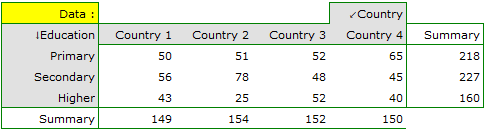
Based on this sample, you would like to find out if there is any dependence between education and country of residence in the analysed population.
Hypotheses:

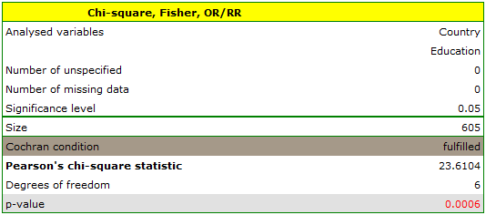

Cochran's condition is satisfied.
The p-value = 0.0006. So, on the basis of the significance level we can draw the conclusion that there is a dependence between education and country of residence in the analysed population.
If we are interested in more precise information about the detected dependencies, we will obtain it by determining multiple comparisons through the options Fisher, Yates and others… and then Multiple column comparisons (RxC) and one of the corrections e.g. Benjamini-Hochberg
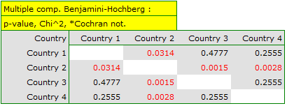
A closer look reveals that only the second country differs from the other countries in educational attainment in a statistically significant way.
The Chi-square test for small tables
These tests are based on the data gathered in the form of a contingency table of 2 features (, ), each of them has 2 possible categories  and
and  (look at the table (\ref{tab_kontyngencji_obser})).
The test for  tables – The Pearson's Chi-square test (Karl Pearson 1900) is constraint of the Chi-square test for (r x c) tables.
The test statistic is defined by:

This statistic asymptotically (for large expected frequencies) has the Chi-square distribution with a 1 degree of freedom.
The settings window with the Chi-square test (2×2) can be opened in Statistics menu → NonParametric tests→Chi-square, Fisher, OR/RR or in ''Wizard''.
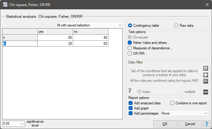
There is a sample consisting of 170 persons ( ). Using this sample, you want to analyse 2 features (=sex, =exam passing). Each of these features occurs in two categories (=f, =m, =yes, =no). Based on the sample you want to get to know, if there is any dependence between sex and exam passing in the above population. The data distribution is presented in the contingency table below:

Hypotheses:

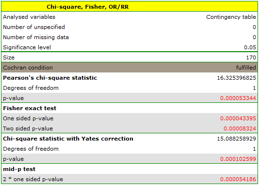
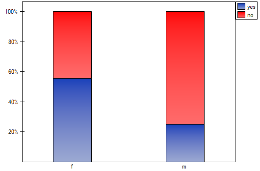
The expectation count table contains no values less than 5. Cochran's condition is satisfied.
At the assumed significance level of all tests performed confirmed the truth of the alternative hypothesis:
- chi-square test, p=0.000053,
- chi-square test with Yeates correction, p=0.000103,
- Fisher's exact test, p=0.000083,
- mid-p test, p=0.000054.
The Fisher's test for large tables
The Fisher test for tables is also called the Fisher-Freeman-Halton test (Freeman G.H., Halton J.H. (1951)12)). This test is an extension on tables of the Fisher's exact test. It defines the exact probability of an occurrence specific distribution of numbers in the table (when we know  and we set the marginal totals).
If you define marginal sums of each row as:

where:
 – observed frequencies in a table,
and the marginal sums of each column as:

then, having defined the marginal sums for the different distributions of the observed frequencies represented by  , you can calculate the
  probabilities:

where

The exact significance level : is the sum of probabilities (calculated for new values ), which are smaller or equal to probability of the table with the initial numbers .
The exact p-value, designated on the basis of the test statistic, is compared with the significance level .
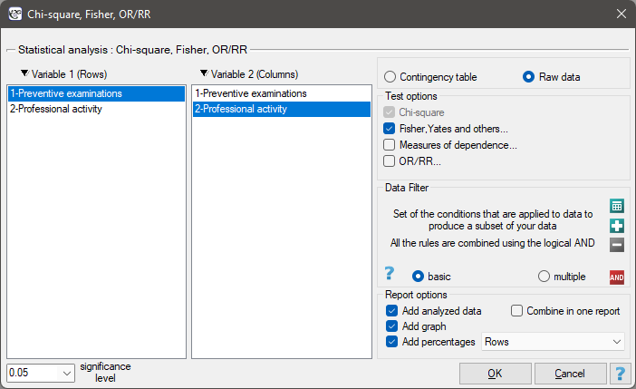
The settings window with the Fisher exact test (RxC) can be opened in Statistics menu → NonParametric tests → Chi-square, Fisher, OR/RR or in ''Wizard''.
Info.
The process of calculation of p-values for this test is based on the algorithm published by Mehta (1986)13).
EXAMPLE (job prevention.pqs file)
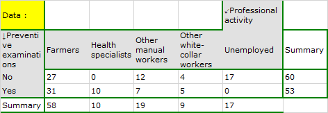
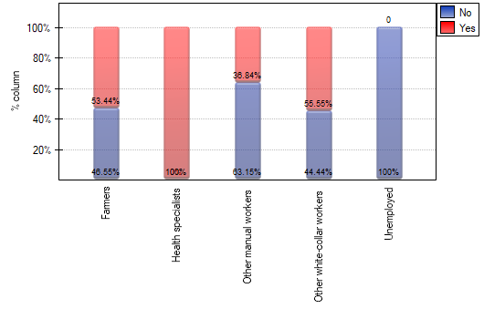
In the population of people living in the rural areas of Komorniki municipality it was examined whether the performance of preventive health examinations depends on the type of occupational activity of the residents. A random sample of 120 people was collected and asked about their education and whether they perform preventive examinations. Complete answers were obtained from 113 persons.
Hypotheses:

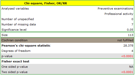
Cochran's condition is not satisfied, thus we should not use the chi-square test.
Value p<0.0001. Therefore, at the significance level we can say that there is a relationship between the performance of preventive examinations and the type of work performed by residents of rural areas of Komorniki municipality.
If we are interested in more precise information about the correlations detected, we will obtain it by determining multiple comparisons through the options Fisher, Yates and others… and then Multiple column comparisons (RxC) and one of the corrections e.g. Benjamini-Hochberg.
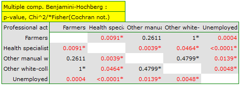
A closer analysis allows us to conclude that health professionals perform preventive examinations significantly more often than the other groups (100% of people in this group performed examinations), and the unemployed significantly less often (no one in this group performed an examination). Farmers, other manual workers and other white-collar workers take preventive examinations in about 50%, which means that these three groups are not statistically significantly different from each other. Part of the p-values obtained in the table is marked with an asterisk, it denotes those results which were obtained by using the Fisher's exact test with Benjamini-Hochberg correction, values not marked with an asterisk are the results of the chi-square test with Benjamini-Hochberg correction, in which Cochran's assumptions were fulfilled.
The Chi-square test corrections for small tables
These tests are based on data collected in the form of a contingency table of 2 features (, ), each of which has possible  categories and (look at the table(\ref{tab_kontyngencji_obser})).
The Chi-square test with the Yate's correction for continuity
The test with the Yate's correction (Frank Yates (1934)14)) is a more conservative test than the Chi-square test (it rejects a null hypothesis more rarely than the test). The correction for continuity guarantees the possibility of taking in all the values of real numbers by a test statistic, according to the distribution assumption.
The test statistic is defined by:

The Fisher test for (2×2) tables
The Fisher test for tables is also called the Fisher exact test (R. A. Fisher (1934)15), (1935)16)). This test enables you to calculate the exact probability of the occurrence of the particular number distribution in a table (knowing and defined marginal sums.

If you know each marginal sum, you can calculate the probability for various configurations of observed frequencies. The exact significance level is the sum of probabilities which are less or equal to the analysed probability.
The mid-p is the Fisher exact test correction. This modified p-value is recommended by many statisticians (Lancaster 196117), Anscombe 198118), Pratt and Gibbons 198119), Plackett 198420), Miettinen 198521) and Barnard 198922), Rothman 200823)) as a method used in decreasing the Fisher exact test conservatism. As a result, using the mid-p the null hypothesis is rejected much more qucikly than by using the Fisher exact test. For large samples a p-value is calculated by using the test with the Yate's correction and the Fisher test gives quite similar results. But a p-value of the test without any correction corresponds with the mid-p.
The p-value of the mid-p is calculated by the transformation of the probability value for the Fisher exact test. The one-sided p-value is calculated by using the following formula:

where:
 – one-sided p-value of mid-p,
 – one-sided p-value of Fisher exact test,
and the two-sided p-value is defined as a doubled value of the smaller one-sided probability:

where:
 – two-sided p-value of mid-p.
The settings window with the chi-square test and its corrections can be opened in Statistics menu → NonParametric tests→Chi-square, Fisher, OR/RR or in ''Wizard''.
The Chi-square test for trend
The test for trend (also called the Cochran-Armitage trend test 24)25))is used to determine whether there is a trend in proportion for particular categories of an analysed variables (features). It is based on the data gathered in the contingency tables of 2 features. The first feature has the possible ordered categories: and the second one has 2 categories:  ,
,  .
The contingency table of
.
The contingency table of  observed frequencies

Basic assumptions:
- measurement on an ordinal scale or on an interval scale,
- an independent model (the second feature - 2 independent groups).
Hypotheses:

where:
 are the proportions
  ,
,  ,…,
,…,  .
.
The test statistic is defined by:
![\begin{displaymath}
\chi^2=\frac{\left[\left(\sum_{i=1}^r i\cdot O_{i1}\right) -C_1\left(\sum_{i=1}^r\frac{i\cdot W_i}{n}\right)\right]^2}{\frac{C_1}{n}\left(1-\frac{C_1}{n}\right)\left[\left(\sum_{i=1}^n i^2 W_i\right)-n\left(\sum_{i=1}^n\frac{i \cdot W_i}{n}\right)^2\right]}.
\end{displaymath}](/lib/exe/fetch.php?media=wiki:latex:/imgd32bd126527cf05771f082e9a0735129.png "LaTeX")
This statistic asymptotically (for large expected frequencies) has the Chi-square distribution with 1 degree of freedom.
The p-value, designated on the basis of the test statistic, is compared with the significance level :
The settings window with the Chi-square test for trend can be opened in Statistics menu → NonParametric tests → Chi-square, Fisher, OR/RR → Chi-square for trend.

EXAMPLE (smoking-education.pqs file)
We examine whether cigarette smoking is related to the education of residents of a village. A sample of 122 people was drawn. The data were recorded in a file. }
We assume that the relationship can be of two types i.e. the more educated people, the more often they smoke or the more educated people, the less often they smoke. Thus, we are looking for an increasing or decreasing trend.
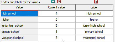
Before proceeding with the analysis, we need to prepare the data, i.e., we need to indicate the order in which the education categories should appear. To do this, from the properties of the Education variable, we select Codes/Labels/Format… and assign the order by specifying consecutive natural numbers. We also assign labels.
Hypotheses:


A p-value=0.0091, which compared to a significance level of =0.05 indicates that the alternative hypothesis that a trend exists is true.

As the graph shows, the more educated people are, the less often they smoke. However, the result obtained by people with junior high school education deviates from this trend. Since there are only two people with lower secondary school education, it did not have much influence on the trend. Due to the very small size of this group, it was decided to repeat the analysis for the combined primary and lower secondary education categories.
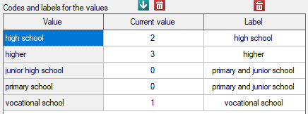
A small value was again obtained p=0.0078 and confirmation of a statistically significant trend.

Because of the decrease in people watching some particular soap opera there was carried out an opinion survey. 100 persons were asked, who has recently started watching this soap opera, and 300 persons were asked, who has watched it regularly from the beginning. They were asked about the level of preoccupation with the character's life. The results are written down in the table below:

The new viewers consist of 25\% of all the analysed viewers. This proportion is not the same for each level of commitment, but looks like this:

Hypotheses:


The p-value=0.0004 which, compared to the significance level =0.05, proves the truth of the alternative hypothesis that there is a trend in the proportions  . As can be seen from the contingency table of the percentages calculated from the sum of the columns, this is a decreasing trend (the more interested the group of viewers is in the fate of the characters of the series, the smaller part of it is made up of new viewers).
The Z test for 2 independent proportions
The test for 2 independent proportions is used in the similar situations as the Chi-square test (2x2). It means, when there are 2 independent samples with the total size of  and
and  , with the 2 possible results to gain (one of the results is distinguished with the size of
  - in the first sample and
  - in the second one). For these samples it is also possible to calculate the distinguished proportions
  and
and  . This test is used to verify the hypothesis informing us that the distinguished proportions
  and
and  in populations, from which the samples were drawn, are equal.
Basic assumptions:
- measurement on a nominal scale - any order is not taken into account,
- large sample sizes.
Hypotheses:

where:
, fraction for the first and the second population.
The test statistic is defined by:

where:
 .
.
The test statistic modified by the continuity correction is defined by:

The Statistic with and without the continuity correction asymptotically (for the large sample sizes) has the normal distribution.
The p-value, designated on the basis of the test statistic, is compared with the significance level :
Apart from the difference between proportions, the program calculates the value of the NNT.
NNT (number needed to treat) – indicator used in medicine to define the number of patients which have to be treated for a certain time in order to cure one person.
NNT is calculated from the formula:

and is quoted when the difference  is positive.
NNH (number needed to harm) – an indicator used in medicine, denotes the number of patients whose exposure to a risk over a specified period of time, results in harm to one person who would not otherwise be harmed. NNH is calculated in the same way as NNT, but is quoted when the difference is negative.
Confidence interval – The narrower the confidence interval, the more precise the estimate. If the confidence interval includes 0 for the difference in proportions and  for the NNT and/or NNH, then there is an indication to treat the result as statistically insignificant
Note
From PQStat version 1.3.0, the confidence intervals for the difference between two independent proportions are estimated on the basis of the Newcombe-Wilson method. In the previous versions it was estimated on the basis of the Wald method.
The justification of the change is as follows:
Confidence intervals based on the classical Wald method are suitable for large sample sizes and for the difference between proportions far from 0 or 1. For small samples and for the difference between proportions close to those extreme values, the Wald method can lead to unreliable results (Newcombe 199826), Miettinen 198527), Beal 198728), Wallenstein 199729)). A comparison and analysis of many methods which can be used instead of the simple Wald method can be found in Newcombe's study (1998)30). The suggested method, suitable also for extreme values of proportions, is the method first published by Wilson (1927)31), extended to the intervals for the difference between two independent proportions.
Note
The confidence interval for NNT and/or NNH is calculated as the inverse of the interval for the proportion, according to the method proposed by Altman (Altman (1998)32)).
The settings window with the Z test for 2 proportions can be opened in Statistics menu → NonParametric tests → Z for 2 independent proportions.
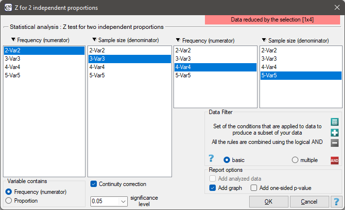
EXAMPLE cont. (sex-exam.pqs file)
You know that  out of all the women in the sample who passed the exam and
  out of all the men in the sample who passed the exam.
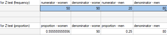
This data can be written in two ways – as a numerator and a denominator for each sample, or as a proportion and a denominator for each sample:
out of all the men in the sample who passed the exam.
This data can be written in two ways – as a numerator and a denominator for each sample, or as a proportion and a denominator for each sample:
Hypotheses:

Note
It is necessary to select the appropriate area (data without headings) before the analysis begins, because usually there are more information in a datasheet. You should also select the option indicating the content of the variable (frequency (numerator) or proportion).
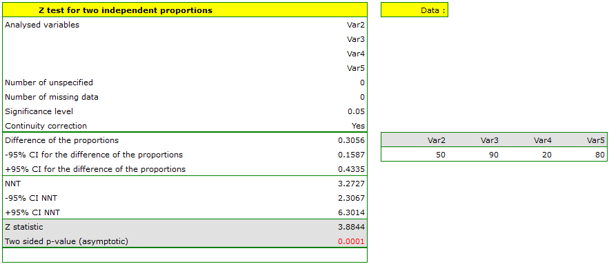
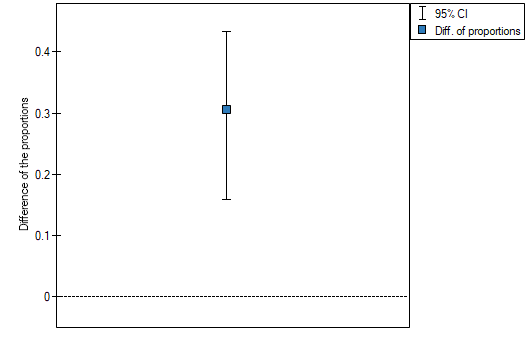
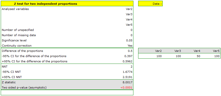
The difference between proportions distinguished in the sample is 30.56%, a 95% and the confidence interval for it  does not contain 0.
Based on the test without the continuity correction as well as on the test with the continuity correction ( p-value < 0.0001), on the significance level =0.05, the alternative hypothesis can be accepted (similarly to the Fisher exact test, its the mid-p corrections, the test and the test with the Yate's correction). So, the proportion of men, who passed the exam is different than the proportion of women, who passed the exam in the analysed population. Significantly, the exam was passed more often by women ( out of all the women in the sample who passed the exam) than by men ( out of all the men in the sample who passed the exam).
EXAMPLE
Let us assume that the mortality rate of a disease is 100\% without treatment and that therapy lowers the mortality rate to 50% – that is the result of 20 years of study. We want to know how many people have to be treated to prevent 1 death in 20 years. To answer that question, two samples of 100 people were taken from the population of the diseased. In the sample without treatment there are 100 patients of whom we know they will all die without the therapy. In the sample with therapy we also have 100 patients of whom 50 will survive. \small{

We will calculate the NNT.
The difference between proportions is statistically significant ( ) but we are interested in the NNT – its value is 2, so the treatment of 2 patients for 20 years will prevent 1 death. The calculated confidence interval value of 95\% should be rounded off to a whole number, wherefore the NNT is 2 to 3 patients.
EXAMPLE
The value of the certain proportion difference in the study comparing the effectiveness of drug 1 vs drug 2 was: difference (95%CI)=-0.08 (-0.27 do 0.11). This negative proportion difference suggests that drug 1 was less effective than drug 2, so its use put patients at risk. Because the proportion difference is negative, the determined inverse is called the NNH, and because the confidence interval contains infinity NNH(95\%CI)= 2.5 (NNH 3.7 to ∞ to NNT 9.1) and goes from NNH to NNT, we should conclude that the result obtained is not statistically significant (Altman (1998)33)).
The Z Test for two dependent proportions
Test for two dependent proportions is used in situations similar to the **McNemar's Test**, i.e. when we have 2 dependent groups of measurements ( i
i  ), in which we can obtain 2 possible results of the studied feature ((+)(–)).

We can also calculated distinguished proportions for those groups  i
i  . The test serves the purpose of verifying the hypothesis that the distinguished proportions and in the population from which the sample was drawn are equal.
Basic assumptions:
- measurement on the nominal - any order is not taken into account,
- large sample size.
Hypotheses:

where:
, fractions for the first and the second measurement.
The test statistic has the form presented below:

The Statistic asymptotically (for the large sample size) has the normal distribution.
The p-value, designated on the basis of the test statistic, is compared with the significance level :
Note
Confidence interval for the difference of two dependent proportions is estimated on the basis of the Newcombe-Wilson method.
The window with settings for Z-Test for two dependent proportions is accessed via the menu Statistics→Nonparametric tests→Z-Test for two dependent proportions.
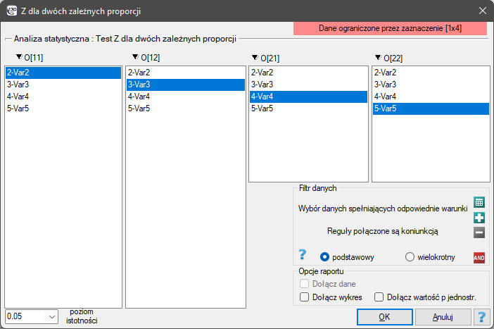
EXAMPLE cont. (opinion.pqs file)
When we limit the study to people who have a specific opinion about the professor (i.e. those who only have a positive or a negative opinion) we will have 152 such students. The data for calculations are:  ,
,  ,
,  ,
,  . We know that
  students expressed a negative opinion before the exam. After the exam the percentage was
  .
.
Hypotheses:

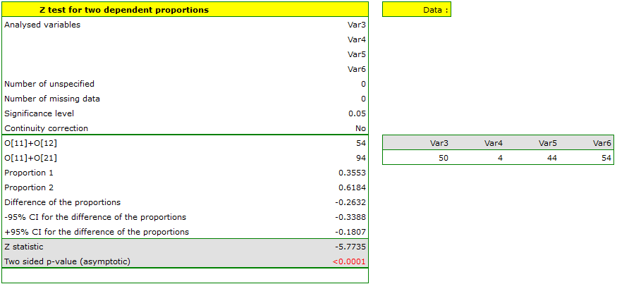
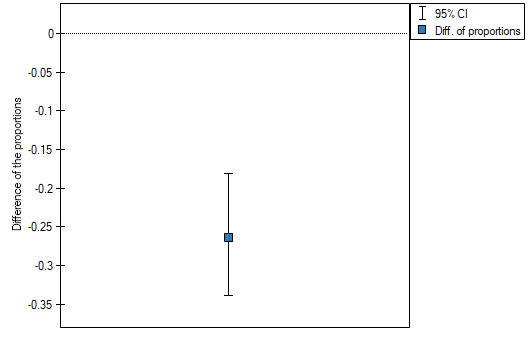
The difference in proportions distinguished in the sample is 26.32%, and the confidence interval of 95% for the sample (18.07%, 33.88%) does not contain 0.
On the basis of a test (p<0.0001), on the significance level of =0.05 (similarly to the case of McNemar's test) we accept the alternative hypothesis. Therefore, the proportion of negative evaluations before the exam differs from the proportion of negative evaluations after the exam. Indeed, after the exam there are more negative evaluations of the professor.
The McNemar test, the Bowker test of internal symmetry
Basic assumptions:
- measurement on a nominal scale - any order is not taken into account,
The McNemar test (NcNemar (1947)34)) is used to verify the hypothesis determining the agreement between the results of the measurements, which were done twice and of an feature (between 2 dependent variables and ). The analysed feature can have only 2 categories (defined here as (+) and (–)). The McNemar test can be calculated on the basis of raw data or on the basis of a contingency table.

Hypotheses:

The test statistic is defined by:

This statistic asymptotically (for large frequencies) has the Chi-square distribution with a 1 degree of freedom.
The p-value, designated on the basis of the test statistic, is compared with the significance level :
The Continuity correction for the McNemar test
This correction is a more conservative test than the McNemar test (a null hypothesis is rejected much more rarely than when using the McNemar test). It guarantees the possibility of taking in all the values of real numbers by the test statistic, according to the distribution assumption. Some sources give the information that the continuity correction should be used always, but some other ones inform, that only if the frequencies in the table are small.
The test statistic with the continuity correction is defined by:

McNemar's exact test
A common general rule for the asymptotic validity of the McNemar chi-square test is the Rufibach assumption, which is that the number of incompatible pairs is greater than 10:  35) when this condition is not satisfied, then we should base the exact probability values of this test 36). The exact probability value of the test is based on a binomial distribution and is a conservative test, so the recommended exact value of the mid-p McNemar test is also given in addition to the exact value of the MnNemar test.
If the study is carried out twice for the same feature and on the same objects – then, odds ratio for the result change (from  to
to  and inversely) is calculated for the table.
The odds for the result change from to is  , and the odds for the result change from to is
  .
.
Odds Ratio ( ) is:
) is:

Confidence interval for the odds ratio is calculated on the base of the standard error:

Note
Additionally, for small sample sizes, the exact range of the confidence interval for the Odds Ratio can be determined37).
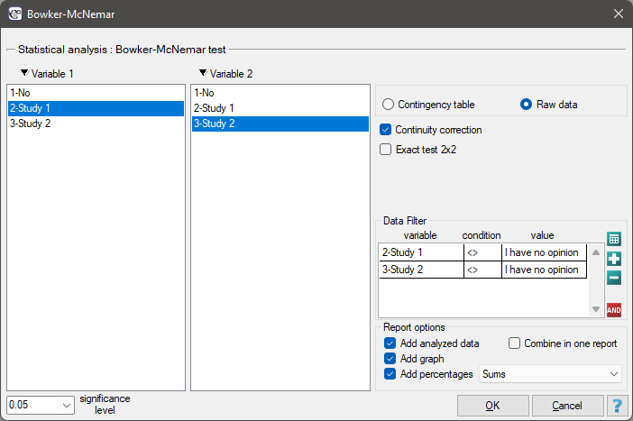
The settings window with the Bowker-McNemar test can be opened in Statistics menu → NonParametric tests → Bowker-McNemar or in ''Wizard''.
The Bowker test of internal symmetry
The Bowker test of internal symmetry (Bowker (1948)38)) is an extension of the McNemar test for 2 variables with more than 2 categories ( ). It is used to verify the hypothesis determining the symmetry of 2 results of measurements executed twice and of feature (symmetry of 2 dependent variables i ). An analysed feature may have more than 2 categories. The Bowker test of internal symmetry can be calculated on the basis of either raw data or a
  contingency table.

Hypotheses:

where  ,
,  ,
,  , so and
  are the frequencies of the symmetrical pairs in the table
The test statistic is defined by:

This statistic asymptotically (for large sample size) has the Chi-square distribution with a number of degrees of freedom calculated using the formula:  .
.
The p-value, designated on the basis of the test statistic, is compared with the significance level :
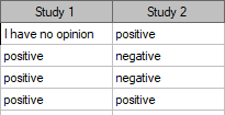
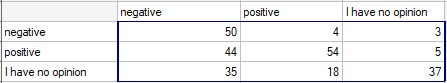
Two different surveys were carried out. They were supposed to analyse students' opinions about the particular academic professor. Both the surveys enabled students to give a positive opinion, a negative and a neutral one. Both surveys were carried out on the basis of the same sample of 250 students. But the first one was carried out the day before an exam done by the professor, and the other survey the day after the exam. There are some data below – in a form of raw rows, and all the data – in the form of a contingency table. Check, if both surveys give the similar results.
Hypotheses:

where, for example, changing the opinion from positive to negative one is symmetrical to changing the opinion from negative to positive one.
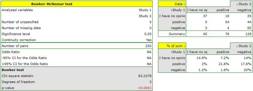
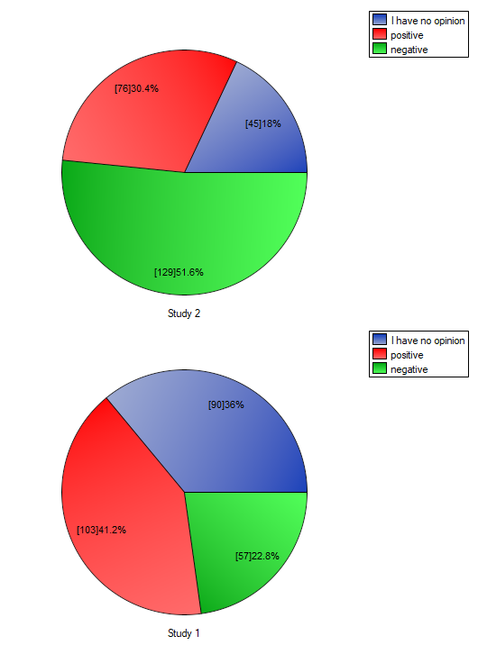
Comparing the p-value for the Bowker test (p-value<0.0001) with the significance level it may be assumed that students changed their opinions. Looking at the table you can see that, there were more students who changed their opinions to negative ones after the exam, than those who changed it to positive ones after the exam. There were also students who did not evaluate the professor in the positive way after the exam any more.
If you limit your analysis only to the people having clear opinions about the professor (positive or negative ones), you can use the McNemar test:
Hypotheses:

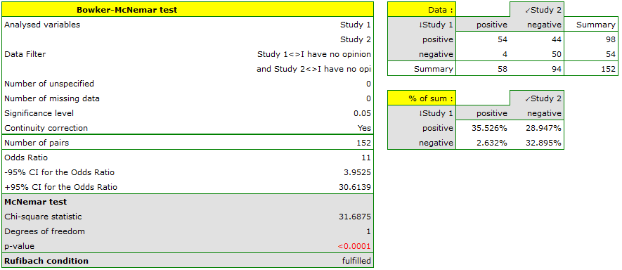
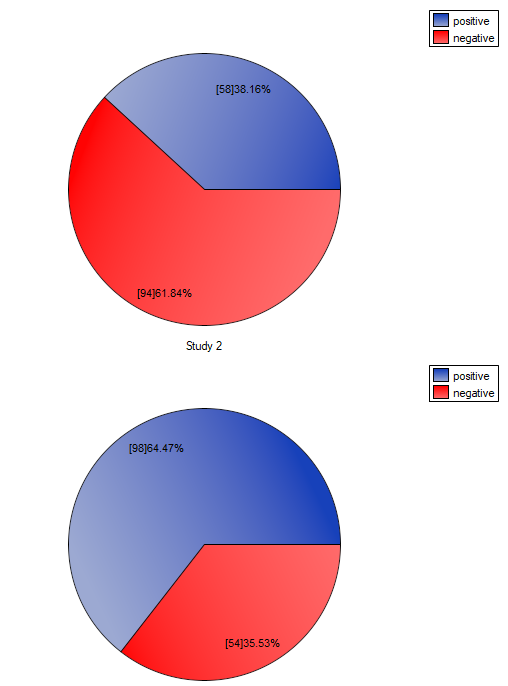
If you compare the p-value, calculated for the McNemar test (p-value < 0.0001), with the significance level , you draw the conclusion that the students changed their opinions. There were much more students, who changed their opinions to negative ones after the exam, than those who changed their opinions to positive ones. The possibility of changing the opinion from positive (before the exam) to negative (after the exam) is eleven  times greater than from negative to positive (the chance to change opinion in the opposite direction is:
  ).
).
1)
Mann H. and Whitney D. (1947), On a test of whether one of two random variables is stochastically larger than the other. Annals of Mathematical Statistics, 1 8 , 5 0 4
2)
, 7)
Wilcoxon F. (1949), Some rapid approximate statistical procedures. Stamford, CT: Stamford Research Laboratories, American Cyanamid Corporation
3)
, 8)
Marascuilo L.A. and McSweeney M. (1977), Nonparametric and distribution-free method for the social sciences. Monterey, CA: Brooks/Cole Publishing Company
4)
, 9)
Fritz C.O., Morris P.E., Richler J.J.(2012), Effect size estimates: Current use, calculations, and interpretation. Journal of Experimental Psychology: General., 141(1):2–18.
5)
, 10)
Cohen J. (1988), Statistical Power Analysis for the Behavioral Sciences, Lawrence Erlbaum Associates, Hillsdale, New Jersey
6)
Wilcoxon F. (1945), Individual comparisons by ranking methods. Biometries, 1, 80-83
11)
Cochran W.G. (1952), The chi-square goodness-of-fit test. Annals of Mathematical Statistics, 23, 315-345
12)
Freeman G.H. and Halton J.H. (1951), Note on an exact treatment of contingency, goodness of fit and other problems of significance. Biometrika 38:141-149
13)
Mehta C.R. and Patel N.R. (1986), Algorithm 643. FEXACT: A Fortran subroutine for Fisher's exact test on unordered r*c contingency tables. ACM Transactions on Mathematical Software, 12, 154–161
14)
Yates F. (1934), Contingency tables involving small numbers and the chi-square test. Journal of the Royal Statistical Society, 1,2 17-235
15)
Fisher R.A. (1934), Statistical methods for research workers (5th ed.). Edinburgh: Oliver and Boyd.
16)
Fisher R.A. (1935), The logic of inductive inference. Journal of the Royal Statistical Society, Series A, 98,39-54
17)
Lancaster H.O. (1961), Significance tests in discrete distributions. Journal of the American Statistical Association 56:223-234
18)
Anscombe F.J. (1981), Computing in Statistical Science through APL. Springer-Verlag, New York
19)
Pratt J.W. and Gibbons J.D. (1981), Concepts of Nonparametric Theory. Springer-Verlag, New York
20)
Plackett R.L. (1984), Discussion of Yates' „Tests of significance for 2×2 contingency tables”. Journal of Royal Statistical Society Series A 147:426-463
21)
Miettinen O.S. (1985), Theoretical Epidemiology: Principles of Occurrence Research in Medicine. John Wiley and Sons, New York
22)
Barnard G.A. (1989), On alleged gains in power from lower p-values. Statistics in Medicine 8:1469-1477
23)
Rothman K.J., Greenland S., Lash T.L. (2008), Modern Epidemiology, 3rd ed. (Lippincott Williams and Wilkins) 221-225
24)
Cochran W.G. (1954), Some methods for strengthening the common chi-squared tests. Biometrics. 10 (4): 417–451
25)
Armitage P. (1955), Tests for Linear Trends in Proportions and Frequencies. Biometrics. 11 (3): 375–386
26)
, 30)
Newcombe R.G. (1998), Interval Estimation for the Difference Between Independent Proportions: Comparison of Eleven Methods. Statistics in Medicine 17: 873-890
27)
Miettinen O.S. and Nurminen M. (1985), Comparative analysis of two rates. Statistics in Medicine 4: 213-226
28)
Beal S.L. (1987), Asymptotic confidence intervals for the difference between two binomial parameters for use with small samples. Biometrics 43: 941-950
29)
Wallenstein S. (1997), A non-iterative accurate asymptotic confidence interval for the difference between two Proportions. Statistics in Medicine 16: 1329-1336
31)
Wilson E.B. (1927), Probable Inference, the Law of Succession, and Statistical Inference. Journal of the American Statistical Association: 22(158):209-212
32)
, 33)
Altman D.G. (1998), Confidence intervals for the number needed to treat. BMJ. 317(7168): 1309–1312
34)
McNemar Q. (1947), Note on the sampling error of the difference between correlated proportions or percentages. Psychometrika, 12, 153-157
35)
Rufibach K. (2010), Assessment of paired binary data; Skeletal Radiology volume 40, pages1–4
36)
Fagerland M.W., Lydersen S., and Laake P. (2013), The McNemar test for binary matched-pairs data: mid-p and asymptotic are better than exact conditional, BMC Med Res Methodol; 13: 91
37)
Liddell F.D.K. (1983), Simplified exact analysis of case-referent studies; matched pairs; dichotomous exposure. Journal of Epidemiology and Community Health; 37:82-84
38)
Bowker A.H. (1948), Test for symmetry in contingency tables. Journal of the American Statistical Association, 43, 572-574
en/statpqpl/porown2grpl/nparpl.txt · ostatnio zmienione: 2022/02/12 16:17 przez admin
Narzędzia strony
Wszystkie treści w tym wiki, którym nie przyporządkowano licencji, podlegają licencji: CC Attribution-Noncommercial-Share Alike 4.0 International
