PQStat - Baza Wiedzy

The Cohen's Kappa coefficient and the test examining its significance

The Cohen's Kappa coefficient (Cohen J. (1960)¹⁾) defines the agreement level of two-times measurements of the same variable in different conditions. Measurement of the same variable can be performed by 2 different observers (reproducibility) or by a one observer twice (recurrence). The $\hat \kappa$ coefficient is calculated for categorial dependent variables and its value is included in a range from -1 to 1. A 1 value means a full agreement, 0 value means agreement on the same level which would occur for data spread in a contingency table randomly. The level between 0 and -1 is practically not used. The negative $\hat \kappa$ value means an agreement on the level which is lower than agreement which occurred for the randomly spread data in a contingency table. The $\hat \kappa$ coefficient can be calculated on the basis of raw data or a $c\times c$ contingency table.

Unweighted Kappa (i.e., Cohen's Kappa) or weighted Kappa can be determined as needed. The assigned weights ( $w_{ij}$ ) refer to individual cells of the contingency table, on the diagonal they are 1 and off the diagonal they belong to the range $<0; 1)$ .

Unweighted Kappa

It is calculated for data, the categories of which cannot be ordered, e.g. data comes from patients, who are divided according to the type of disease which was diagnosed, and these diseases cannot be ordered, e.g. pneumonia $(1)$ , bronchitis $(2)$ and other $(3)$ . In such a situation, one can check the concordance of the diagnoses given by the two doctors by using unweighted Kappa, or Cohen's Kappa. Discordance of pairs ${(1), (3)}$ and ${(1), (2)}$ will be treated equivalently, so the weights off the diagonal of the weight matrix will be zeroed.

Weighted Kappa

In situations where data categories can be sorted, e.g., data comes from patients who are divided by the lesion grade into: no lesion $(1)$ , benign lesion $(2)$ , suspected cancer $(3)$ , cancer $(4)$ , one can build the concordance of the ratings given by the two radiologists taking into account the possibility of sorting. The ratings of ${(1), (4)}$ than ${(1), (2)}$ may then be considered as more discordant pairs of ratings. For this to be the case, so that the order of the categories affects the compatibility score, the weighted Kappa should be determined.

The assigned weights can be in linear or quadratic form.

Linear weights (Cicchetti, 1971²⁾) – calculated according to the formula:

$\begin{displaymath} w_{ij}=1-\frac{|i-j|}{c-1}. \end{displaymath}$

The greater the distance from the diagonal of the matrix the smaller the weight, with the weights decreasing proportionally. Example weights for matrices of size 5×5 are shown in the table:

$\begin{tabular}{|c|c|c|c|c|} \hline1&0.75&0.5&0.25&0\\\hline 0.75&1&0.75&0.5&0.25\\\hline 0.5&0.75&1&0.75&0.5\\\hline 0.25&0.5&0.75&1&0.75\\\hline 0&0.25&0.5&0.75&1\\\hline \end{tabular}$

Square weights (Cohen, 1968³⁾) – calculated according to the formula:

$\begin{displaymath} w_{ij}=1-\frac{(i-j)^2}{(c-1)^2}. \end{displaymath}$

The greater the distance from the diagonal of the matrix, the smaller the weight, with weights decreasing more slowly at closer distances from the diagonal and more rapidly at farther distances. Example weights for matrices of size 5×5 are shown in the table:

$\begin{tabular}{|c|c|c|c|c|} \hline1&0.9375&0.75&0.4375&0\\\hline 0.9375&1&0.9375&0.75&0.4375\\\hline 0.75&0.9375&1&0.9375&0.75\\\hline 0.4375&0.75&0.9375&1&0.9375\\\hline 0&0.4375&0.75&0.9375&1\\\hline \end{tabular}$

Quadratic scales are of greater interest because of the practical interpretation of the Kappa coefficient, which in this case is the same as the intraclass correlation coefficient ⁴⁾. To determine the Kappa coefficient compliance, the data are presented in the form of a table of observed counts $O_{ij}$ , and this table is transformed into a probability contingency table $p_{ij}=O_{ij}/n$ .

The Kappa coefficient ( $\hat \kappa$ ) is expressed by the formula: $\begin{displaymath} \hat \kappa=\frac{P_o-P_e}{1-P_e}, \end{displaymath}$

where:

$P_o=\sum_{i=1}^c\sum_{j=1}^c w_{ij}p_{ij}$ ,

$P_e=\sum_{i=1}^c\sum_{j=1}^c w_{ij}p_{i.}p_{.i}$ ,

$p_{i.}$ , $p_{.i}$ - total sums of columns and rows of the probability contingency table.

Note

$\hat \kappa$ denotes the concordance coefficient in the sample, while $\kappa$ in the population.

The standard error for Kappa is expressed by the formula:

$\begin{displaymath} SE_{\hat \kappa}=\frac{1}{(1-P_e)\sqrt{n}}\sqrt{\sum_{i=1}^{c}\sum_{j=1}^{c}p_{i.}p_{.j}[w_{ij}-(\overline{w}_{i.}+(\overline{w}_{.j})]^2-P_e^2} \end{displaymath}$

where:

$\overline{w}_{i.}=\sum_{j=1}^{c}p_{.j}w_{ij}$ ,

$\overline{w}_{.j}=\sum_{i=1}^{c}p_{i.}w_{ij}$ .

The Z test of significance for the Cohen's Kappa ( $\hat \kappa$ ) (Fleiss,2003⁵⁾) is used to verify the hypothesis informing us about the agreement of the results of two-times measurements $X^{(1)}$ and $X^{(2)}$ features $X$ and it is based on the $\hat \kappa$ coefficient calculated for the sample.

Basic assumptions:

measurement on a nominal scale (unweighted Kappa) or on a ordinal scale (unweighted Kappa).

Hypotheses:

$\begin{array}{cl} \mathcal{H}_0: & \kappa= 0, \\ \mathcal{H}_1: & \kappa \ne 0. \end{array}$

The test statistic is defined by:

$\begin{displaymath} Z=\frac{\hat \kappa}{SE_{\kappa_{distr}}}, \end{displaymath}$

Where:

$\displaystyle{SE_{\kappa_{distr}}=\frac{1}{(1-P_e)\sqrt{n}}\sqrt{\sum_{i=1}^c\sum_{j=1}^c p_{ij}[w_{ij}-(\overline{w}_{i.}+\overline{w}_{.j})(1-\hat \kappa)]^2-[\hat \kappa-P_e(1-\hat \kappa)]^2}}$ .

The $Z$ statistic asymptotically (for a large sample size) has the normal distribution.

The p-value, designated on the basis of the test statistic, is compared with the significance level $\alpha$ :

$\begin{array}{ccl} $ if $ p \le \alpha & \Longrightarrow & $ reject $ \mathcal{H}_0 $ and accept $ \mathcal{H}_1, \\ $ if $ p > \alpha & \Longrightarrow & $ there is no reason to reject $ \mathcal{H}_0. \\ \end{array}$

The settings window with the test of Cohen's Kappa significance can be opened in Statistics menu → NonParametric tests → Kappa-Cohen or in ''Wizard''.

EXAMPLE (diagnosis.pqs file)

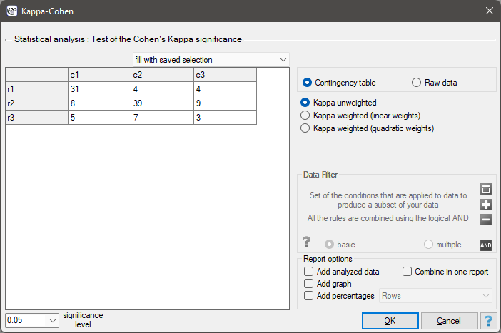
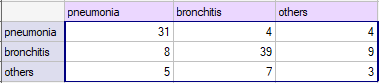
You want to analyse the compatibility of a diagnosis made by 2 doctors. To do this, you need to draw 110 patients (children) from a population. The doctors treat patients in a neighbouring doctors' offices. Each patient is examined first by the doctor A and then by the doctor B. Both diagnoses, made by the doctors, are shown in the table below.

Hypotheses:

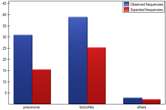
$\begin{array}{cl} \mathcal{H}_0: & \kappa= 0, \\ \mathcal{H}_1: & \kappa \ne 0. \end{array}$

We could analyse the agreement of the diagnoses using just the percentage of the compatible values. In this example, the compatible diagnoses were made for 73 patients (31+39+3=73) which is 66.36% of the analysed group. The kappa coefficient introduces the correction of a chance agreement (it takes into account the agreement occurring by chance).

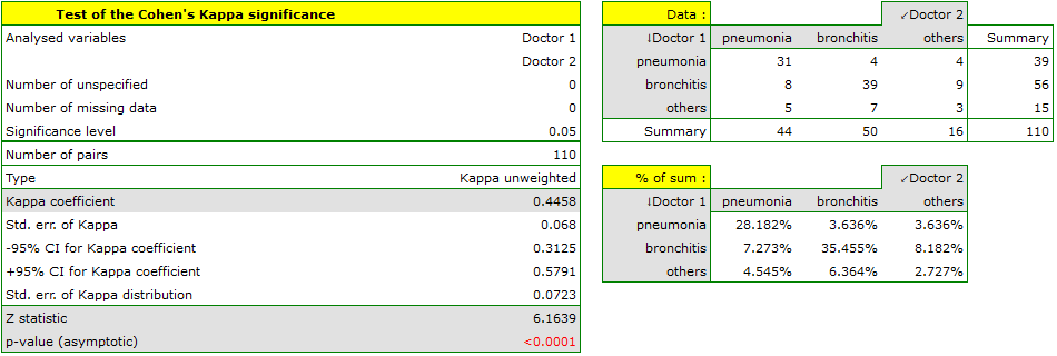
The agreement with a chance adjustment $\hat \kappa=44.58%$ is smaller than the one which is not adjusted for the chances of an agreement.

The p<0.0001. Such result proves an agreement between these 2 doctors' opinions, on the significance level $\alpha=0.05$ ,.

EXAMPLE (radiology.pqs file)

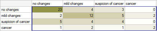
Radiological imaging assessed liver damage in the following categories: no changes (1), mild changes (2), suspicion of cancer $(3)$ , cancer $(4)$ . The evaluation was done by two independent radiologists based on a group of 70 patients. We want to check the concordance of the diagnosis.

Hypotheses:

$\begin{array}{cl} \mathcal{H}_0: & \kappa= 0, \\ \mathcal{H}_1: & \kappa \ne 0. \end{array}$

Because the diagnosis is issued on an ordinal scale, an appropriate measure of concordance would be the weighted Kappa coefficient.

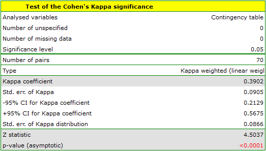
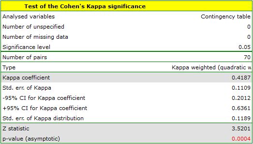
Because the data are mainly concentrated on the main diagonal of the matrix and in close proximity to it, the coefficient weighted by the linear weights is lower ( $\hat \kappa= 0.39$ ) than the coefficient determined for the quadratic weights ( $\hat \kappa= 0.42$ ). In both situations, this is a statistically significant result (at the $\alpha=0.05$ significance level), p<0.0001.

If there was a large disagreement in the ratings concerning the two extreme cases and the pair: (no change and cancer) located in the upper right corner of the table occurred far more often, e.g., 15 times, then such a large disagreement would be more apparent when using quadratic weights (the Kappa coefficient would drop dramatically) than when using linear weights.

¹⁾

Cohen J. (1960), A coefficient of agreement for nominal scales. Educational and Psychological Measurement, 10,3746

²⁾

Cicchetti D. and Allison T. (1971), A new procedure for assessing reliability of scoring eeg sleep recordings. American Journal EEG Technology, 11, 101-109

³⁾

Cohen J. (1968), Weighted kappa: nominal scale agreement with provision for scaled disagreement or partial credit. Psychological Bulletin, 70, 213-220

⁴⁾

Fleiss J.L., Cohen J. (1973), The equivalence of weighted kappa and the intraclass correlation coeffcient as measure of reliability. Educational and Psychological Measurement, 33, 613-619

⁵⁾

Fleiss J.L., Levin B., Paik M.C. (2003), Statistical methods for rates and proportions. 3rd ed. (New York: John Wiley) 598-626

PQStat - Baza Wiedzy

Narzędzia użytkownika

Narzędzia witryny

Pasek boczny

The Cohen's Kappa coefficient and the test examining its significance

Narzędzia strony