PQStat - Baza Wiedzy

The Q-Cochran ANOVA

The Q-Cochran analysis of variance, based on the Q-Cochran test, is described by Cochran (1950)¹⁾. This test is an extended McNemar test for $k\geq2$ dependent groups. It is used in hypothesis verification about symmetry between several measurements $X^{(1)}, X^{(2)},..., X^{(k)}$ for the $X$ feature. The analysed feature can have only 2 values - for the analysis, there are ascribed to them the numbers: 1 and 0.

Basic assumptions:

measurement on a nominal scale (dichotomous variables – it means the variables of two categories),
a dependent model.

Hypotheses:

$\begin{array}{cl} \mathcal{H}_0: & $all the "incompatible" observed frequencies are equal,$ \\ \mathcal{H}_1: & $not all the "incompatible" observed frequencies are equal,$ \end{array}$

where:

„incompatible” observed frequencies – the observed frequencies calculated when the value of the analysed feature is different in several measurements.

The test statistic is defined by: $\begin{displaymath} Q=\frac{(k-1)\left(kC-T^2\right)}{kT-R} \end{displaymath}$

where:

$T=\sum_{i=1}^n\sum_{j=1}^kx_{ij}$ ,

$R=\sum_{i=1}^n\left(\sum_{j=1}^kx_{ij}\right)^2$ ,

$C=\sum_{j=1}^k\left(\sum_{i=1}^nx_{ij}\right)^2$ ,

$x_{ij}$ – the value of $j$ -th measurement for $i$ -th object (so 0 or 1).

This statistic asymptotically (for large sample size) has the Chi-square distribution with a number of degrees of freedom calculated using the formula: $df=k-1$ .

The p-value, designated on the basis of the test statistic, is compared with the significance level $\alpha$ :

$\begin{array}{ccl} $ if $ p \le \alpha & \Longrightarrow & $ reject $ \mathcal{H}_0 $ and accept $ \mathcal{H}_1, \\ $ if $ p > \alpha & \Longrightarrow & $ there is no reason to reject $ \mathcal{H}_0. \\ \end{array}$

The POST-HOC tests

Introduction to the contrasts and the POST-HOC tests was performed in the unit, which relates to the one-way analysis of variance.

The Dunn test

For simple comparisons (frequency in particular measurements is always the same).

Hypotheses:

Example - simple comparisons (for the difference in proportion in a one chosen pair of measurements):

$\begin{array}{cl} \mathcal{H}_0: & $the chosen "incompatible" observed frequencies are equal,$ \\ \mathcal{H}_1: & $the chosen "incompatible" observed frequencies are different.$ \end{array}$

[i] The value of critical difference is calculated by using the following formula:

$\begin{displaymath} CD=Z_{\frac{\alpha}{c}}\sqrt{2\frac{kT-R}{n^2k(k-1)}}, \end{displaymath}$

where:

$\displaystyle Z_{\frac{\alpha}{c}}$ - is the critical value (statistic) of the normal distribution for a given significance level $\alpha$ corrected on the number of possible simple comparisons $c$ .

</WRAP

[ii] The test statistic is defined by:

$\begin{displaymath} Z=\frac{\sum_{j=1}^k c_jp_j}{\sqrt{2\frac{kT-R}{n^2k(k-1)}}}, \end{displaymath}$

where:

$p_j$ – the proportion $j$ -th measurement $(j=1,2,...k)$ ,

The test statistic asymptotically (for large sample size) has the normal distribution, and the p-value is corrected on the number of possible simple comparisons $c$ .

The settings window with the Cochran Q ANOVA can be opened in Statistics menu→ NonParametric tests→Cochran Q ANOVA or in ''Wizard''.

Note

This test can be calculated only on the basis of raw data.

EXAMPLE(test.pqs file)

We want to compare the difficulty of 3 test questions. To do this, we select a sample of 20 people from the analysed population. Every person from the sample answers 3 test questions. Next, we check the correctness of answers (an answer can be correct or wrong). In the table, there are following scores:

$\begin{tabular}{|c|c|c|c|} \hline No.&question 1 answer &question 2 answer &question 3 answer \\\hline 1&correct&correct&wrong\\ 2&wrong&correct&wrong\\ 3&correct&correct&correct\\ 4&wrong&correct&wrong\\ 5&wrong&correct&wrong\\ 6&wrong&correct&correct\\ 7&wrong&wrong&wrong\\ 8&wrong&correct&wrong\\ 9&correct&correct&wrong\\ 10&wrong&correct&wrong\\ 11&wrong&wrong&wrong\\ 12&wrong&wrong&correct\\ 13&wrong&correct&wrong\\ 14&wrong&wrong&correct\\ 15&correct&wrong&wrong\\ 16&wrong&wrong&wrong\\ 17&wrong&correct&wrong\\ 18&wrong&correct&wrong\\ 19&wrong&wrong&wrong\\ 20&correct&correct&wrong\\\hline \end{tabular}$

Hypotheses:

$\begin{array}{cl} \mathcal{H}_0: & $The individual questions received the same number of correct answers,$\\ & $in the analysed population,$\\ \mathcal{H}_1: & $There are different numbers of correct and wrong answers in individual test questions, $\\ & $in the analysed population.$ \end{array}$

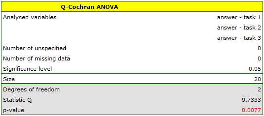
Comparing the p value p=0.0077 with the significance level $\alpha=0.05$ we conclude that individual test questions have different difficulty levels. We resume the analysis to perform POST-HOC test by clicking , and in the test option window, we select POST-HOC Dunn.

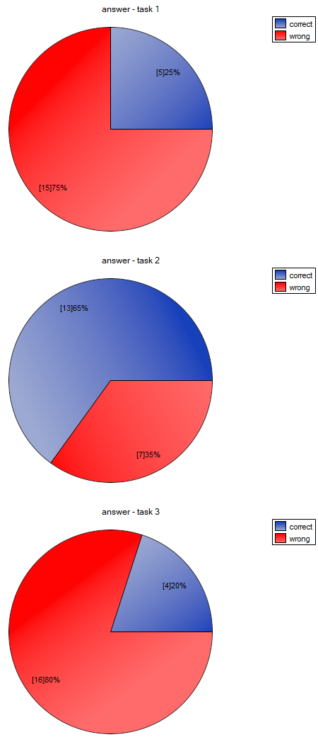
The carried out POST-HOC analysis indicates that there are differences between the 2-nd and 1-st question and between questions 2-nd and 3-th. The difference is because the second question is easier than the first and the third ones (the number of correct answers the first question is higher).

¹⁾

Cochran W.G. (1950), The comparison ofpercentages in matched samples. Biometrika, 37, 256-266

PQStat - Baza Wiedzy

Narzędzia użytkownika

Narzędzia witryny

Pasek boczny

The Q-Cochran ANOVA

Narzędzia strony