PQStat - Baza Wiedzy

Spis treści

Non-parametric tests

Non-parametric tests

The Kruskal-Wallis ANOVA

The Kruskal-Wallis one-way analysis of variance by ranks (Kruskal 1952 ¹⁾; Kruskal and Wallis 1952 ²⁾) is an extension of the U-Mann-Whitney test on more than two populations. This test is used to verify the hypothesis that there is no shift in the compared distributions, i.e., most often the insignificant differences between medians of the analysed variable in ( $k\geq2$ ) populations (but you need to assume, that the variable distributions are similar - comparison of rank variances can be checked using Conover's rank test).

Additional analyses:

it is possible to test for a trend in the arrangement of the groups under study by performing the Jonckheere-Terpstra test for trend.

Basic assumptions:

measurement on an ordinal scale or on an interval scale,
an independent model.

Hypotheses:

$\begin{array}{cl} \mathcal{H}_0: & \phi_1=\phi_2=...=\phi_k,\\ \mathcal{H}_1: & $not all $\phi_j$ are equal $(j=1,2,...,k)$,$ \end{array}$

where:

$\phi_1,\phi_2,...\phi_k$ distributions of the analysed variable of each population.

The test statistic is defined by:

$\begin{displaymath} H=\frac{1}{C}\left(\frac{12}{N(N+1)}\sum_{j=1}^k\left(\frac{\left(\sum_{i=1}^{n_j}R_{ij}\right)^2}{n_j}\right)-3(N+1)\right), \end{displaymath}$

where:

$N=\sum_{j=1}^k n_j$ ,

$n_j$ – samples sizes $(j=1,2,...k)$ ,

$R_{ij}$ – ranks ascribed to the values of a variable for $(i=1,2,...n_j)$ , $(j=1,2,...k)$ ,

$\displaystyle C=1-\frac{\sum(t^3-t)}{N^3-N}$ – correction for ties,

$t$ – number of cases included in a tie.

The formula for the test statistic $H$ includes the correction for ties $C$ . This correction is used, when ties occur (if there are no ties, the correction is not calculated, because of $C=1$ ).

The $H$ statistic asymptotically (for large sample sizes) has the Chi-square distribution with the number of degrees of freedom calculated using the formula: $df = (k - 1)$ .

The p-value, designated on the basis of the test statistic, is compared with the significance level $\alpha$ :

$\begin{array}{ccl} $ if $ p \le \alpha & \Longrightarrow & $ reject $ \mathcal{H}_0 $ and accept $ \mathcal{H}_1, \\ $ if $ p > \alpha & \Longrightarrow & $ there is no reason to reject $ \mathcal{H}_0. \\ \end{array}$

The POST-HOC tests

Introduction to the contrasts and the POST-HOC tests was performed in the unit, which relates to the one-way analysis of variance.

The Dunn test

For simple comparisons, equal-size groups as well as unequal-size groups.

The Dunn test (Dunn 1964³⁾) includes a correction for tied ranks (Zar 2010⁴⁾) and is a test corrected for multiple testing. The Bonferroni or Sidak correction is most commonly used here, although other, newer corrections are also available, described in more detail in Multiple comparisons.

Example - simple comparisons (comparing 2 selected median / mean ranks with each other):

$\begin{array}{cc} \mathcal{H}_0: & \theta_j=\theta_{j+1},\\ \mathcal{H}_1: & \theta_j \neq \theta_{j+1}. \end{array}$

[i] The value of critical difference is calculated by using the following formula:

$\begin{displaymath} CD=Z_{\frac{\alpha}{c}}\sqrt{\frac{N(N+1)}{12}\left(\sum_{j=1}^k \frac{c_j^2}{n_j}\right)}, \end{displaymath}$

where:

$\displaystyle Z_{\frac{\alpha}{c}}$ - is the critical value (statistic) of the normal distribution for a given significance level $\alpha$ corrected on the number of possible simple comparisons $c$ .

[ii] The test statistic is defined by:

$\begin{displaymath} Z=\frac{\sum_{j=1}^k c_j\overline{R}_j}{\sqrt{\frac{N(N+1)}{12}\left(\sum_{j=1}^k \frac{c_j^2}{n_j}\right)}}, \end{displaymath}$

where:

$\overline{R}_j$ – mean of the ranks of the $j$ -th group, for $(j=1,2,...k)$ ,

The formula for the test statistic $Z$ includes a correction for tied ranks. This correction is applied when tied ranks are present (when there are no tied ranks this correction is not calculated because $\sum(t^3-t)=0$ ).

The test statistic asymptotically (for large sample sizes) has the normal distribution, and the p-value is corrected on the number of possible simple comparisons $c$ .

Conover-Inman test

The non-parametric equivalent of Fisher LSD⁵⁾, used for simple comparisons of both groups of equal and different sizes.

[i] The value of critical difference is calculated by using the following formula:

$\begin{displaymath} CD=\sqrt{F_{\alpha,1,N-k}}\cdot\sqrt{S^2\frac{N-1-H}{N-k}\sum_{j=1}^k \frac{c_j^2}{n_j}}, \end{displaymath}$

where:

$\displaystyle S^2=\frac{1}{N-1}\left(\sum_{j=1}^k\sum_{i=1}^{n_j}R_{ij}^2-N\frac{(N+1)^2}{4}\right)$

$\displaystyle F_{\alpha,1,N-k}$ is the critical value (statistic) Snedecor's F distribution for a given significance level $\alpha$ and for degrees of freedom respectively: 1 i $N-k$ .

[ii] The test statistic is defined by:

$\begin{displaymath} t=\frac{\sum_{j=1}^k c_j\overline{R}_j}{\sqrt{S^2\frac{N-1-H}{N-k}\sum_{j=1}^k \frac{c_j^2}{n_j}}}, \end{displaymath}$

where:

$\overline{R}_j$ – The mean ranks of the $j$ -th group, for $(j=1,2,...k)$ ,

This statistic follows a t-Student distribution with $N-k$ degrees of freedom.

The settings window with the Kruskal-Wallis ANOVA can be opened in Statistics menu→NonParametric tests →Kruskal-Wallis ANOVA or in ''Wizard''.

EXAMPLE (jobSatisfaction.pqs)

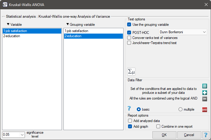
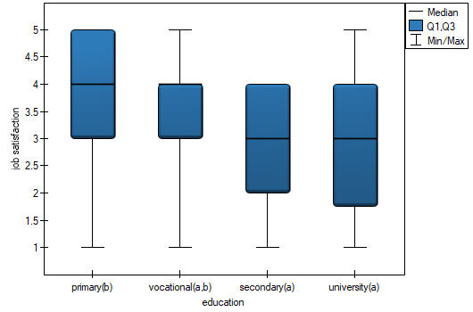
A group of 120 people was interviewed, for whom the occupation is their first job obtained after receiving appropriate education. The respondents rated their job satisfaction on a five-point scale, where:

1- unsatisfying job,

2- job giving little satisfaction,

3- job giving an average level of satisfaction,

4- job that gives a fairly high level of satisfaction,

5- job that is very satisfying.

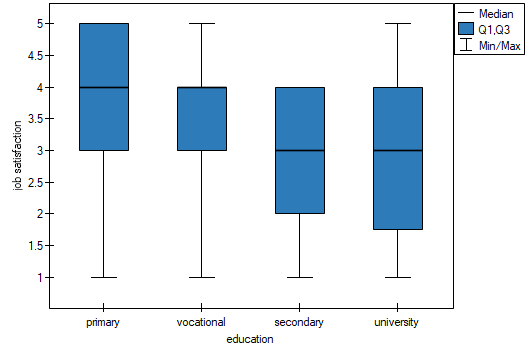
We will test whether the level of reported job satisfaction does not change for each category of education.

Hypotheses:

$\begin{array}{cl} \mathcal{H}_0: & $the level of job satisfaction is the same for each education category,$\\ \mathcal{H}_1: & $at least one education category (one population) $ \\ &$has different levels of job satisfaction.$ \end{array}$

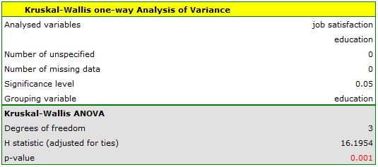
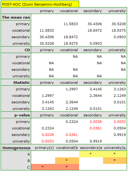
The obtained value of p=0.001 indicates a significant difference in the level of satisfaction between the compared categories of education. Dunn's POST-HOC analysis with Bonferroni's correction shows that significant differences are between those with primary and secondary education and those with primary and tertiary education. Slightly more differences can be confirmed by selecting the stronger POST-HOC Conover-Iman.

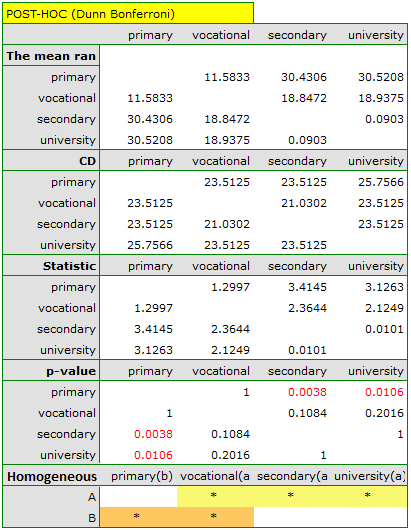
In the graph showing medians and quartiles we can see homogeneous groups determined by the POST-HOC test. If we choose to present Dunn's results with Bonferroni correction we can see two homogeneous groups that are not completely distinct, i.e. group (a) - people who rate job satisfaction lower and group (b)- people who rate job satisfaction higher. Vocational education belongs to both of these groups, which means that people with this education evaluate job satisfaction quite differently. The same description of homogeneous groups can be found in the results of the POST-HOC tests.

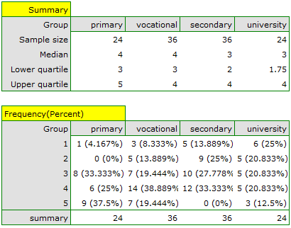
We can provide a detailed description of the data by selecting descriptive statistics in the analysis window and indicating to add counts and percentages to the description.

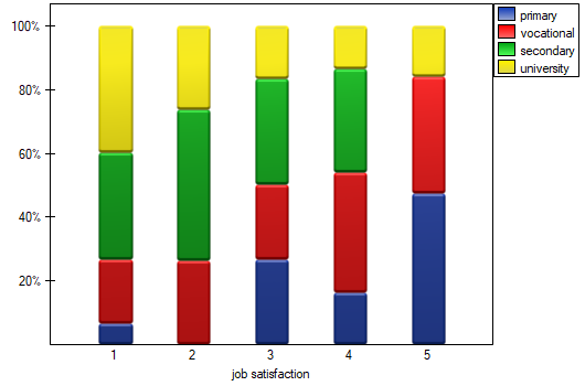
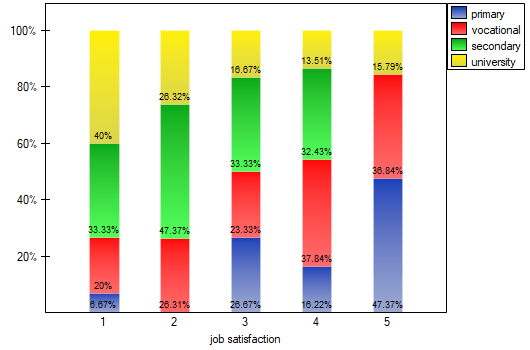
We can also show the distribution of responses in a column plot.

2022/02/09 12:56

The Jonckheere-Terpstra test for trend

The Jonckheere-Terpstra test for ordered alternatives described independently by Jonckheere (1954) ⁶⁾ an be calculated in the same situation as the Kruskal-Wallis ANOVA , as it is based on the same assumptions. The Jonckheere-Terpstra test, however, captures the alternative hypothesis differently - indicating in it the existence of a trend for successive populations.

Hypotheses are simplified to medians:

$\begin{array}{cl} \mathcal{H}_0: & \theta_1=\theta_2=...=\theta_k,\\ \mathcal{H}_1: & \theta_1\geq\theta_2\geq...\geq\theta_k, $ with at least one strict inequality$ \end{array}$

Note

The term: „with at least one strict inequality” written in the alternative hypothesis of this test means that at least the median of one population should be greater than the median of another population in the order specified.

The test statistic has the form:

$\begin{displaymath} Z=\frac{L-\left[\frac{N^2-\sum_{j=1}^kn_j^2}{4}\right]}{SE} \end{displaymath}$

where:

$L=$ – sum of $l_{ij}$ values obtained for each pair of compared populations,

$l_{ij}$ – number of results higher than a preset value in the next occurring group,

$SE=\sqrt{\frac{A}{72}+\frac{B}{36N(N-1)(N-2)}+\frac{C}{8N(N-1)}}$ ,

$A=N(N-1)(2N+5)-\sum_{j=1}^kn_j(n_j-1)(2n_j+5)-\sum_{l=1}^gt_l(t_l-1)(2t_l+5)$ ,

$B=\sum_{j=1}^kn_j(n_j-1)(n_j-2)\cdot\sum_{l=1}^gt_l(t_l-1)(t_l-2)$ ,

$C=\sum_{j=1}^kn_j(n_j-1)\cdot\sum_{l=1}^gt_l(t_l-1)$ ,

$g$ – number of groups of different tied ranks,

$t_l$ – umber of cases included in the tied rank,

$N=\sum_{j=1}^k n_j$ ,

$n_j$ – sample sizes for $(j=1,2,...k)$ .

Note

To be able to perform a trend analysis, the expected order of the populations must be indicated by assigning consecutive natural numbers.

The formula for the test statistic $Z$ includes the correction for ties. This correction is applied when tied ranks are present (when there are no tied ranks the test statistic formula reduces to the original Jonckheere-Terpstra formula without this correction).

The statistic $Z$ has asymptotically (for large samples) normal distribution.

With the expected direction of the trend known, the alternative hypothesis is one-sided and the one-sided p-value is interpreted. The interpretation of the two-sided p-value means that the researcher does not know (does not assume) the direction of the possible trend.

The p-value, designated on the basis of the test statistic, is compared with the significance level $\alpha$ :

$\begin{array}{ccl} $ if $ p \le \alpha & \Longrightarrow & $ reject $ \mathcal{H}_0 $ and accept $ \mathcal{H}_1, \\ $ if $ p > \alpha & \Longrightarrow & $ there is no reason to reject $ \mathcal{H}_0. \\ \end{array}$

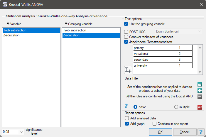
The settings window with the Jonckheere-Terpstra test for trend can be opened in Statistics menu→NonParametric tests→Kruskal-Wallis ANOVA or in ''Wizard''.

EXAMPLE cont. (jobSatisfaction.pqs file)

It is suspected that better educated people have high job demands, which may reduce the satisfaction level of the first job, which often does not meet such demands. Therefore, it is worthwhile to conduct a trend analysis.

Hypotheses:

$\begin{array}{cl} \mathcal{H}_0: & $No indicated trend in satisfaction with first job,$\\ \mathcal{H}_1: & $There is an indicated trend in the level of satisfaction with the first job.$ \end{array}$

To do this, we resume the analysis with the button, select the Jonckheere-Terpstra trend test option, and assign successive natural numbers to the education categories.

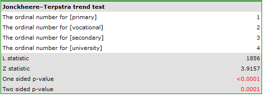
The obtained one-sided value p<0.0001 and is less than the set significance level $\alpha=0.05$ , which speaks in favor of a trend actually occurring consistent with the researcher's expectations.

We can also confirm the existence of this trend by showing the percentage distribution of responses obtained.

2022/02/09 12:56

The Conover ranks test of variance

Conover squared ranks test is used, similarly to Fisher-Snedecor test (for $k=2$ ), Levene test and Brown-Forsythe test (for $k>=2$ ) to verify the hypothesis of similar variation of the tested variable in several populations. It is the non-parametric counterpart of the tests indicated above, by that it does not assume normality of the data distribution and is based on the ranks⁷⁾.However, this test examines variation and therefore distances to the mean, so the basic condition for its use is:

measurement on an interval scale,

Hypotheses:

$\begin{array}{cc} \mathcal{H}_0: & $the dispersion of the data in the populations being compared is the same, $\\ \mathcal{H}_1: & $at least two populations differ in the amount of data dispersion$. \end{array}$

The test statistic has the form:

$\begin{displaymath} \chi^2=\frac{1}{D^2}\left(\sum_{j=1}^k\frac{S_j^2}{n_j}-N\overline{S}^2\right) \end{displaymath}$

where:

$N=n_1+n_2+...+n_k$ ,

$n_j$ – individual group sizes,

$S_j$ –sum of ranks squares in $j$ -th group,

$\overline{S}=\frac{1}{N}\sum_{j=1}^k\S_j$ – mean of all ranks squares,

$D^2=\frac{1}{N-1}\left(\sum_{ji=1}^NR_i^4-N\overline{S}^2\right)$ ,

$R_i$ – ranks for values representing the distance of the measurement from the mean of a given group.

This statistic has a Chi-squaredistribution with $k-1$ degrees of freedom.

The p-value, designated on the basis of the test statistic, is compared with the significance level $\alpha$ :

$\begin{array}{ccl} $ if $ p \le \alpha & \Longrightarrow & $ reject $ \mathcal{H}_0 $ and accept $ \mathcal{H}_1, \\ $ if $ p > \alpha & \Longrightarrow & $ there is no reason to reject $ \mathcal{H}_0. \\ \end{array}$

The settings window with the Conover ranks test of variance can be opened in Statistics menu→NonParametric tests→Kruskal-Wallis ANOVA, option Conover ranks test of variance or textsf{Statistics} menu→NonParametric tests→Mann-Whitney, option Conover ranks test of variance.

EXAMPLE(surgeryMethod.pqs file)

Patients have been prepared for spinal surgery. The patients will be operated on by one of three methods. Preliminary allocation of each patient to each type of surgery has been made. At a later stage we intend to compare the condition of the patients after the surgeries, therefore we want the groups of patients to be comparable. They should be similar in terms of the height of the interbody space (WPMT) before surgery. The similarity should concern not only the average values but also the differentiation of the groups.

The distribution of the data was checked

It is found that for the two methods, the WPMT operation exhibits deviations from normality, largely caused by skewness of the data. Further comparative analysis will be conducted using the Kruskal-Wallis test to compare whether the level of WPMT differs between the methods, and the Conover test to indicate whether the spread of WPMT scores is similar in each method.

Hypotheses for Conover's variance test:

$\begin{array}{cl} \mathcal{H}_0: & $The diversity (scope) of WPMT is the same for each method of operation,$\\ \mathcal{H}_1: & $WPMT diversity (range) is higher/lower for at least one method of operation.$ \end{array}$

Hypotheses for Kruskal-Wallis test:

$\begin{array}{cl} \mathcal{H}_0: & $WPMT level is the same for each operation method,$\\ \mathcal{H}_1: & $WPMT level is higher/lower for at least one method of operation.$ \end{array}$

First, the value of Conover's test of variance is interpreted, which indicates statistically significant differences in the ranges of the groups compared (p=0.0022). From the graph, we can conclude that the differences are mainly in group 3. Since differences in WPMT were detected, the interpretation of the result of the Kruskal-Wallis test comparing the level of WPMT for these methods should be cautious, since this test is sensitive to heterogeneity of variance. Although the Kruskal-Wallis test showed no significant differences (p=0.2057), it is recommended that patients with low WPMT (who were mainly assigned to surgery with method B) be more evenly distributed, i.e. to see if they could be offered surgery with method A or C. After reassignment of patients, the analysis should be repeated.

2022/02/09 12:56

The Friedman ANOVA

The Friedman repeated measures analysis of variance by ranks – the Friedman ANOVA - was described by Friedman (1937)⁸⁾. This test is used when the measurements of an analysed variable are made several times ( $k\geq2$ ) each time in different conditions. It is also used when we have rankings coming from different sources (form different judges) and concerning a few ( $k\geq2$ ) objects, but we want to assess the grade of the rankings agreement.

Iman Davenport (1980⁹⁾) has shown that in many cases the Friedman statistic is overly conservative and has made some modification to it. This modification is the non-parametric equivalent of the ANOVA for dependent groups which makes it now recommended for use in place of the traditional Friedman statistic.

Additional analyses:

It is possible to take missing data into account by using the Accept missing data option, calculating Durbin ANOVA or Skillings-Mack ANOVA;
it is possible to test the trend in the arrangement of the studied groups by performing Page test for trend.

Basic assumptions:

measurement on an ordinal scale or on an interval scale,
a dependent model.

Hypotheses relate to the equality of the sum of ranks for successive measurements ( $R_{j}$ ) or are simplified to medians ( $\theta_j$ )

$\begin{array}{cl} \mathcal{H}_0: & \theta_1=\theta_2=...=\theta_k,\\ \mathcal{H}_1: & $not all $\theta_j$ are equal $(j=1,2,...,k)$,$ \end{array}$

where:

$\theta_1,\theta_2,...\theta_k$ medians for an analysed features, in the following measurements from the examined population.

Two test statistics are determined: the Friedman statistic and the Iman-Davenport modification of this statistic.

The Friedman statistic has the form:

$\begin{displaymath} T_1=\frac{1}{C}\left(\frac{12}{nk(k+1)}\left(\sum_{j=1}^k\left(\sum_{i=1}^n R_{ij}\right)^2\right)-3n(k+1)\right), \end{displaymath}$

where:

$n$ – sample size,

$R_{ij}$ – ranks ascribed to the following measurements $(j=1,2,...k)$ , separately for the analysed objects $(i=1,2,...n)$ ,

$\displaystyle C=1-\frac{\sum(t^3-t)}{n(k^3-k)}$ – correction for ties,

$t$ – number of cases included in a tie.

The Iman-Davenport modification of the Friedman statistic has the form:

$\begin{displaymath} T_2=\frac{(n_j-1)T_1}{n_j(k-1)-T_1} \end{displaymath}$

The formula for the test statistic $T_1$ and $T_2$ includes the correction for ties $C$ . This correction is used, when ties occur (if there are no ties, the correction is not calculated, because of $C=1$ ).

The $T_1$ statistic has asymptotically (for large sample sizes) has the Chi-square distribution with $df=k - 1$ degrees of freedom.

The statistic $T_2$ follows the Snedecor's F distribution with $df_1=k-1$ i $df_2=(n_j-1)(k-1)$ degrees of freedem.

The p-value, designated on the basis of the test statistic, is compared with the significance level $\alpha$ :

$\begin{array}{ccl} $ if $ p \le \alpha & \Longrightarrow & $ reject $ \mathcal{H}_0 $ and accept $ \mathcal{H}_1, \\ $ if $ p > \alpha & \Longrightarrow & $ there is no reason to reject $ \mathcal{H}_0. \\ \end{array}$

The POST-HOC tests

Introduction to the contrasts and the POST-HOC tests was performed in the unit, which relates to the one-way analysis of variance.

The Dunn test

For simple comparisons (frequency in particular measurements is always the same).

The Dunn test (Dunn 1964¹⁰⁾) is a corrected test due to multiple testing. The Bonferroni or Sidak correction is most commonly used here, although other, newer corrections are also available and are described in more detail in the Multiple Comparisons section.

Hypotheses:

Example - simple comparisons (comparison of 2 selected medians):

$\begin{array}{cc} \mathcal{H}_0: & \theta_j=\theta_{j+1},\\ \mathcal{H}_1: & \theta_j \neq \theta_{j+1}. \end{array}$

[i] The value of critical difference is calculated by using the following formula:

$\begin{displaymath} CD=Z_{\frac{\alpha}{c}}\sqrt{\frac{k(k+1)}{6n}}, \end{displaymath}$

where:

$\displaystyle Z_{\frac{\alpha}{c}}$ - is the critical value (statistic) of the normal distribution for a given significance level $\alpha$ corrected on the number of possible simple comparisons $c$ .

[ii] The test statistic is defined by:

$\begin{displaymath} Z=\frac{\sum_{j=1}^k c_jR_j}{\sqrt{\frac{k(k+1)}{6n}}}, \end{displaymath}$

where:

$\overline{R}_j$ – mean of the ranks of the $j$ -th measurement, for $(j=1,2,...k)$ ,

The test statistic asymptotically (for large sample size) has normal distribution, and the p-value is corrected on the number of possible simple comparisons $c$ .

Conover-Inman test

Non-parametric equivalent of Fisher LSD¹¹⁾, sed for simple comparisons (counts across measurements are always the same).

[i] he value of critical difference is calculated by using the following formula:

$\begin{displaymath} CD=\sqrt{F_{\alpha,1,df_2}}\cdot\sqrt{\frac{2\left(n_jA-\sum_{j=1}^tR_j^k\right)}{(n_j-1)(k-1)}}, \end{displaymath}$

where:

$\displaystyle A=\sum_{i=1}^{n_j}\sum_{j=1}^kR_{ij}^2$ – sum of squares for ranks,

$\displaystyle F_{\alpha,1,df_2}$ to critical value (statistic) Snedecor's F distribution for a given significance level $\alpha$ and for degrees of freedom respectively: 1 and $df_2$ .

[ii] The test statistic is defined by:

$\begin{displaymath} t=\frac{\sum_{j=1}^k c_jR_j}{\sqrt{\frac{2\left(n_jA-\sum_{j=1}^tR_j^k\right)}{(n_j-1)(k-1)}}}, \end{displaymath}$

where:

$R_j$ – the sum of ranks of $j$ th measurement, for $(j=1,2,...k)$ ,

The test statistic hast-Student distribution with $df_2$ degrees of freedem.

The settings window with the Friedman ANOVA can be opened in Statistics menu→NonParametric tests →Friedman ANOVA, trend test or in ''Wizard''

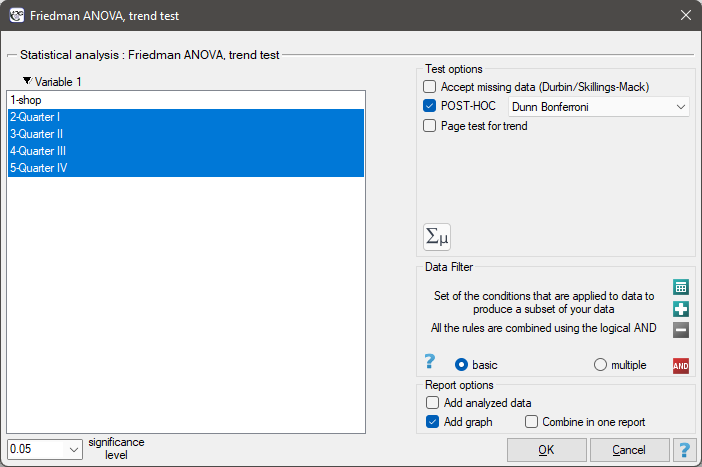
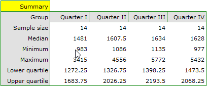
EXAMPLE (chocolate bar.pqs file)

Quarterly sale of some chocolate bar was measured in 14 randomly chosen supermarkets. The study was started in January and finished in December. During the second quarter, the billboard campaign was in full swing. Let's check if the campaign had an influence on the advertised chocolate bar sale.

$\begin{tabular}{|c|c|c|c|c|} \hline Shop&Quarter I&Quarter II&Quarter III&Quarter IV\\\hline SK1&3415&4556&5772&5432\\ SK2&1593&1937&2242&2794\\ SK3&1976&2056&2240&2085\\ SK4&1526&1594&1644&1705\\ SK5&1538&1634&1866&1769\\ SK6&983&1086&1135&1177\\ SK7&1050&1209&1245&977\\ SK8&1861&2087&2054&2018\\ SK9&1714&2415&2361&2424\\ SK10&1320&1621&1624&1551\\ SK11&1276&1377&1522&1412\\ SK12&1263&1279&1350&1490\\ SK13&1271&1417&1583&1513\\ SK14&1436&1310&1357&1468\\\hline \end{tabular}$

Hypotheses:

$\begin{array}{cl} \mathcal{H}_0: & $there is a lack of significant difference in sale values, in the compared $\\ & $quarters, in the population represented by the whole sample, $\\ \mathcal{H}_1: & $the difference in sale values, between at least 2 quarters, is significant,$\\ & $in the population represented by the whole sample.$ \end{array}$

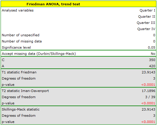
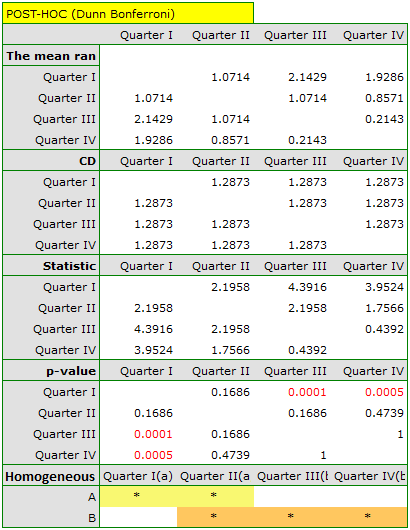
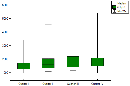
Comparing the p-value of the Friedman test (as well as the p-value of the Iman-Davenport correction of the Friedman test) with a significance level $\alpha=0.05$ , we find that sales of the bar are not the same in each quarter. The POST-HOC Dunn analysis performed with the Bonferroni correction indicates differences in sales volumes pertaining to quarters I and III and I and IV, and an analogous analysis performed with the stronger Conover-Iman test indicates differences between all quarters except quarters III and IV.

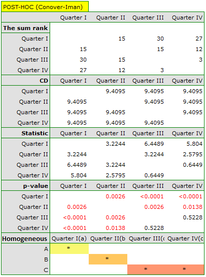
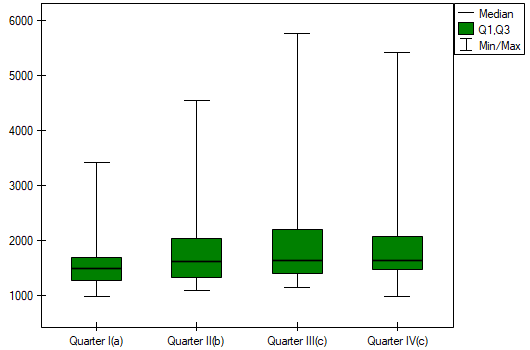
In the graph, we presented homogeneous groups determined by the Conover-Iman test.

We can provide a detailed description of the data by selecting Descriptive statistics in the analysis window .

If the data were described by an ordinal scale with few categories, it would be useful to present it also in numbers and percentages. In our example, this would not be a good method of description.

2022/02/09 12:56

The Page test for trend

The Page test for ordered alternative described in 1963 by Page E. B. ¹²⁾ can be computed in the same situation as Friedman's ANOVA, since it is based on the same assumptions. However, Page's test captures the alternative hypothesis differently - indicating that there is a trend in subsequent measurements.

Hypotheses involve equality of the sum of ranks for successive measurements or are simplified to medians:

$\begin{array}{cl} \mathcal{H}_0: & \theta_1=\theta_2=...=\theta_k,\\ \mathcal{H}_1: & \theta_1\geq\theta_2\geq...\geq\theta_k, $ with at least one strict inequality$ \end{array}$

Note

The term: „with at least one strict inequality” written in the alternative hypothesis of this test means that at least one median should be greater than the median of another group of measurements in the order specified.

The test statistic has the form:

$\begin{displaymath} Z=\frac{L-\left[\frac{nk(k+1)^2}{4}\right]}{\sqrt{\frac{n(k^3-k)^2}{144(k-1)}}} \end{displaymath}$

where:

$L=\sum_{j=1}^kR_jc_j$ ,

$R_j$ – the sum of ranks of $j$ th measurement,

$c_j$ –the weight for $j$ -th measurement informing about the natural order of this measurement among other measurements (weights are consecutive natural numbers).

Note

In order to perform a trend analysis, the expected ordering of measurements must be indicated by assigning consecutive natural numbers to successive measurement groups. These numbers are treated as weights in the analysis $c_1$ , $c_2$ , …, $c_k$ .

The formula for the test statistic $Z$ does not include a correction for ties, making it somewhat more conservative when tied ranks are present. However, using a correction for tied ranks for this test is not recommended.

The statistic $Z$ has asymptotically (for large sample) normal distribution.

With the expected direction of the trend known, the alternative hypothesis is one-sided and the one-sided p-value is interpreted. Interpreting a two-sided p-value means that the researcher does not know (does not assume) the direction of the possible trend.

The p-value, designated on the basis of the test statistic, is compared with the significance level $\alpha$ :

$\begin{array}{ccl} $ if $ p \le \alpha & \Longrightarrow & $ reject $ \mathcal{H}_0 $ and accept $ \mathcal{H}_1, \\ $ if $ p > \alpha & \Longrightarrow & $ there is no reason to reject $ \mathcal{H}_0. \\ \end{array}$

The settings window with the Page test for trend can be opened in Statistics menu→NonParametric tests →Friedman ANOVA, trend test or in ''Wizard''

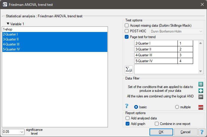
EXAMPLE cont. (chocolate bar.pqs file)

The expected result of the intensive advertising campaign conducted by the company is a steady increase in sales of the offered bar.

Hypotheses:

$\begin{array}{cl} \mathcal{H}_0: & $no indicated trend in bar sales,$\\ \mathcal{H}_1: & $there is an indicated trend in bar sales.$ \end{array}$

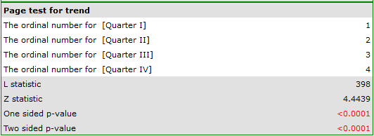
Comparing a one-sided p<0.0001 with a significance level $\alpha=0.05$ , we find that the campaign produced the expected trend of increased product sales.

2022/02/09 12:56

The Durbin's ANOVA (missing data)

Durbin's analysis of variance of repeated measurements for ranks was proposed by Durbin (1951)¹³⁾. This test is used when measurements of the variable under study are made several times – a similar situation in which Friedman'sANOVA is used. The original Durbin test and the Friedman test give the same result when we have a complete data set. However, Durbin's test has an advantage – it can also be calculated for an incomplete data set. At the same time, data deficiencies cannot be located arbitrarily, but the data must form a so-called balanced and incomplete block:

the number of measurements for each object is $k$ ( $k \leq t$ ),
each measurement is made on $r$ objects ( $r \leq b$ ),
the number of objects for which the same pair of measurements was taken simultaneously is constant and equal to $\lambda$ .

where:

$t$ – total number of considered measurements,

$b$ – total number of examined objects.

Basic assumptions:

measurement on an ordinal scale or on an interval scale,
a dependent model.

Hypotheses involve equality of the sum of ranks for successive measurements ( $R_{j}$ ) or are simplified to medians ( $\theta_j$ ):

$\begin{array}{cl} \mathcal{H}_0: & \theta_1=\theta_2=...=\theta_k,\\ \mathcal{H}_1: & $not all $\theta_j$ are equal $(j=1,2,...,k)$,$ \end{array}$

Two test statistics of the following form are determined:

$\begin{displaymath} T_1=\frac{(t-1)\left[\sum_{j=1}^tR_j^2-tC\right]}{A-C}, \end{displaymath}$

$\begin{displaymath} T_2=\frac{T_1/(t-1)}{(b(k-1)-T_1)/(bk-b-t+1)}, \end{displaymath}$

where:

$R_{j}$ – sum of ranks for successive measurements $(j=1,2,...t)$ ,

$R_{ij}$ – ranks assigned to successive measurements, separately for each of the studied objects $(i=1,2,...b)$ ,

$\displaystyle A=\sum_{i=1}^b\sum_{j=1}^tR_{ij}^2$ – sum of squared ranks,

$\displaystyle C=\frac{bk(k+1)^2}{4}$ – correction coefficient.

The formula for $T_1$ and $T_2$ statistics includes a correction for tied ranks.

For complete data, the $T_1$ statistic is the same as the Friedman test. It has asymptotically (for large sample sizes) Chi-square distribution with $df=t - 1$ degrees of freedom.

The $T_2$ statistic is the equivalent of Friedman's Iman-Davenport ANOVA adjustment, so it follows Snedecor's F distribution with $df_1=t-1$ i $df_2=bk-b-t+1$ degrees of freedom. It is now considered to be more precise than the $T_1$ statistic and is recommended for use with the $T_1$ statistic¹⁴⁾.

The p-value, designated on the basis of the test statistic, is compared with the significance level $\alpha$ :

$\begin{array}{ccl} $ if $ p \le \alpha & \Longrightarrow & $ reject $ \mathcal{H}_0 $ and accept $ \mathcal{H}_1, \\ $ if $ p > \alpha & \Longrightarrow & $ there is no reason to reject $ \mathcal{H}_0. \\ \end{array}$

Testy POST-HOC

Introduction to the contrasts and the POST-HOC tests was performed in the unit, which relates to the one-way analysis of variance.

Conover-Inman test

Used for simple comparisons (the counts in each measurement are always the same).

Hypotheses:

Example - simple comparisons (comparing 2 selected medians / rank sums between each other):

$\begin{array}{cc} \mathcal{H}_0: & \theta_j=\theta_{j+1},\\ \mathcal{H}_1: & \theta_j \neq \theta_{j+1}. \end{array}$

[ii] The value of critical difference is calculated by using the following formula:

$\begin{displaymath} CD=t_{1-\alpha /2, bk-b-t+1}\sqrt{\frac{(A-C)2r}{bk-b-t+1}\left(1-\frac{T_1}{b(k-1)}\right)}, \end{displaymath}$

where:

$t_{1-\alpha /2, bk-b-t+1}$ – is the [wartosc_krytyczna|critical value (statistic) of the t-Student distribution for a given significance level $\alpha$ and $df=bk-b-t+1$ degrees of freedom.

[ii] The test statistic has the form:

$\begin{displaymath} t=\frac{\sum_{j=1}^k c_jR_j}{\sqrt{\frac{(A-C)2r}{bk-b-t+1}\left(1-\frac{T_1}{b(k-1)}\right)}}, \end{displaymath}$

The test statistic has t-Student distribution with $df=bk-b-t+1$ degrees of freedom.

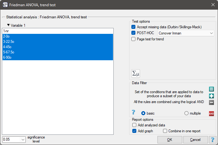
The settings window with the Durbin's ANOVA can be opened in Statistics menu→NonParametric tests →Friedman ANOVA, trend test or in ''Wizard''

Note

For records with missing data to be taken into account, you must check the Accept missing data option. Empty cells and cells with non-numeric values are treated as missing data. Only records with more than one numeric value will be analyzed.

EXAMPLE (mirror.pqs file)

An experiment was conducted among 20 patients in a psychiatric hospital (Ogilvie 1965)¹⁵⁾. This experiment involved drawing straight lines according to a presented pattern. The pattern represented 5 lines drawn at different angles ( $0^o, 22.5^o, 45^o, 67.5^o, 90^o$ ) relative to the indicated center. The patients' task was to reproduce the lines while having their hand covered. The time at which the patient drew the line was recorded as the result of the experiment. Ideally, each patient would draw a line from all angles, but elapsed time and fatigue would have a significant impact on performance. In addition, it is difficult to keep the patient interested and willing to cooperate for an extended period of time. Therefore, the project was planned and conducted in balanced and incomplete blocks. Each of the 20 patients traced a line at two angles (there were five possible angles). Thus, each angle was drawn eight times. The time at which each patient drew a line at a given angle was recorded in the table.

$\begin{tabular}{|c||c|c|c|c|c|} \hline patient number &$0^o$&$22.5^o$&$45^o$&$67.5^o$&$90^o$\\\hline 1&7&15&&&\\ 2&20&&72&&\\ 3&8&&&26&\\ 4&33&&&&36\\ 5&7&16&&&\\ 6&&68&67&&\\ 7&&33&&64&\\ 8&&34&&&12\\ 9&10&&96&&\\ 10&&29&59&&\\ 11&&&17&9&\\ 12&&&100&&15\\ 13&16&&&32&\\ 14&&19&&32&\\ 15&&&36&39&\\ 16&&&&44&54\\ 17&16&&&&38\\ 18&&17&&&12\\ 19&&&37&&11\\ 20&&&&56&6\\ \hline \end{tabular}$

We want to see if the time taken to draw each line is completely random, or if there are lines that took more or less time to draw.

Hypotheses:

$\begin{array}{cl} \mathcal{H}_0: & $there is no significant difference between the time $\\ & $taken by patients to draw each line, $\\ \mathcal{H}_1: & $at least one line is drawn in shorter/longer time.$ \end{array}$

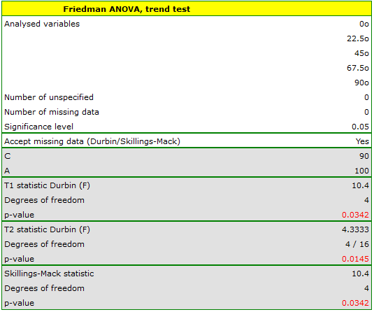
Comparing the p=0.0145 for the $T_2$ statistic (or the p=0.0342 for the $T_1$ statistic) with the $\alpha=0.05$ significance level, we find that the lines are not drawn at the same time. The POST-HOC analysis performed indicates that there is a difference in the time taken to draw the line at angle $0^o$ . It is drawn faster than the lines at the angle of $22.5^o$ , $45^o$ and $67.5^o$ .

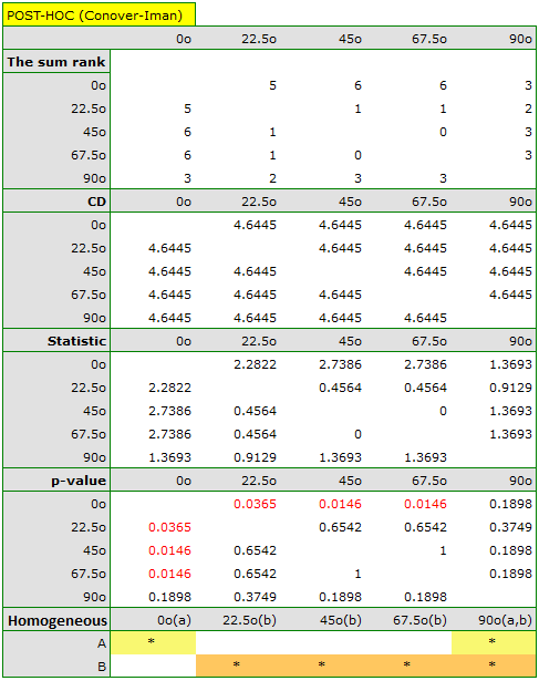
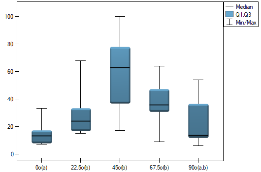
The graph shows homogeneous groups indicated by the post-hoc test.

2022/02/09 12:56

The Skillings-Mack ANOVA (missing data)

The analysis of variance of repeated measures for Skillings-Mack ranks was proposed by Skillings and Mack in 1981 ¹⁶⁾. t is a test that can be used when there are missing data, but the missing data need not occur in any particular setting. However, each site must have at least two observations. If there are no tied ranks and no gaps are present it is the same as the Friedman's ANOVA, and if data gaps are present in a balanced arrangement it corresponds to the results of Durbin's ANOVA.

Basic assumptions: Basic assumptions:

measurement on an ordinal scale or on an interval scale,
a dependent model.

Hypotheses relate to the equality of the sum of ranks for successive measurements ( $R_{j}$ ) or are simplified to medians ( $theta_j$ )

$\begin{array}{cl} \mathcal{H}_0: & \theta_1=\theta_2=...=\theta_k,\\ \mathcal{H}_1: & $nie wszystkie $\theta_j$ są sobie równe $(j=1,2,...,k)$,$ \end{array}$

The test statistic has the form:

$\begin{displaymath} \chi^2=A\Sigma_0^{-1}A^T \end{displaymath}$

where:

$A=(A_1,A_2,...,A_{k-1}$

$A_j=\sum_{i=1}^n\sqrt{\frac{12}{s_i+1}}\left(R_{ij}-\frac{s_i+1}{2}\right)$ ,

$s_i$ – number of observations for $i$ -th object,

$R_{ij}$ – ranks assigned to successive measurements ( $j = 1, 2, ...k$ ), separately for each study object ( $i = 1, 2, ...n$ ), with ranks for missing data equal to the average rank for the object,

$\Sigma_0$ – matrix determining the covariances for $A$ at the truth of $\mathcal{H}_0$ ¹⁷⁾.

When each pair of measurements occurs simultaneously for at least one observation, this statistic has asymptotically (for large sample sizes) the Chi-square distribution with $k-1$ degrees of freedom.

The p-value, designated on the basis of the test statistic, is compared with the significance level $\alpha$ :

$\begin{array}{ccl} $ if $ p \le \alpha & \Longrightarrow & $ reject $ \mathcal{H}_0 $ and accept $ \mathcal{H}_1, \\ $ if $ p > \alpha & \Longrightarrow & $ there is no reason to reject $ \mathcal{H}_0. \\ \end{array}$

The settings window with the Skillings-Mack ANOVA can be opened in Statistics menu→NonParametric tests →Friedman ANOVA, trend test or in ''Wizard''

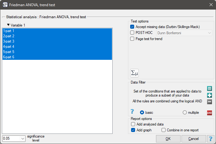
Note

For records with missing data to be taken into account, you must check the Accept missing data option. Empty cells and cells with non-numeric values are treated as missing data. Only records containing more than one numeric value will be analyzed.

EXAMPLE (polling.pqs file)

A certain university teacher, wanting to improve the way he conducted his classes, decided to verify his teaching skills. In several randomly selected student groups, during the last class, he asked them to fill in a short anonymous questionnaire. The survey consisted of six questions about how the six specified parts of the material were illustrated. The students could rate it on a 5-point scale, where 1 - the way of presenting the material was completely incomprehensible, 5 - a very clear and interesting way of illustrating the material. The data obtained in this way turned out to be incomplete due to the fact that students did not answer questions about the part of the material they were absent on. In the 30-person group completing the survey, only 15 students provided complete responses. Performing an analysis that does not account for data gaps (in this case, a Friedman analysis) will have limited power by cutting the group size so drastically and will not lead to the detection of significant differences. Data gaps were not planned for and are not present in the balanced block, so this task cannot be performed using Durbin's analysis along with his POST-HOC test.

Hypotheses:

$\begin{array}{cl} \mathcal{H}_0: & $there is no significant difference in the evaluations of the different parts of the material by$\\ & $studentów, $\\ \mathcal{H}_1: & $at least one part of the material is assessed differently by students.$ \end{array}$

The results of the ANOVA Skillings-Mack analysis are presented in the following report:

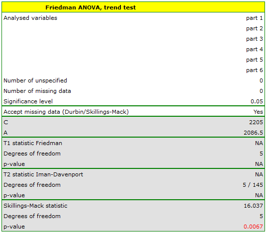
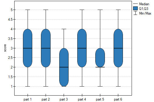
The $p$ value obtained should be treated with caution due to possible tied ranks. However, for this study, the p=0.0067 is well below the accepted significance level of $\alpha=0.05$ , indicating that significant differences exist. The differences in responses can be observed in the graph; however, there is no POST-HOC analysis available for this test.

2022/02/09 12:56

The Chi-square test for multidimensional contingency tables

Basic assumptions:

measurement on a nominal scale - any order is not taken into account,
an independent model,
large expected frequencies (according to the Cochran interpretation (1952)¹⁸⁾.

Hypotheses:

$\begin{array}{cl} \mathcal{H}_0: & O_{ij...}=E_{ij...} $ for all categories,$\\ \mathcal{H}_1: & O_{ij...} \neq E_{ij...} $ for at least one category,$ \end{array}$

where:

$O_{ij...}$ and $E_{ij...}$ $-$ observed frequencies in a contingency table and the corresponding expected frequencies.

The test statistic is defined by:

$\begin{displaymath} \chi^2=\sum_{i=1}^r\sum_{j=1}^c\sum...\sum\frac{(O_{ij...}-E_{ij...})^2}{E_{ij...}}. \end{displaymath}$

This statistic asymptotically (for large expected frequencies) has the Chi-square distribution with a number of degrees of freedom calculated using the formula: $df = (r - l)(c - 1)(l - 1) + (r- l)(c- 1) + (r- 1)(l- 1) + (c- 1)(l- 1)$ - for 3-dimensional tables.

The p-value, designated on the basis of the test statistic, is compared with the significance level $\alpha$ :

$\begin{array}{ccl} $ if $ p \le \alpha & \Longrightarrow & $ reject $ \mathcal{H}_0 $ and accept $ \mathcal{H}_1, \\ $ if $ p > \alpha & \Longrightarrow & $ there is no reason to reject $ \mathcal{H}_0. \\ \end{array}$

The settings window with the Chi-square (multidimensional) test can be opened in Statistics menu → NonParametric tests (unordered categories)→Chi-square (multidimensional) or in ''Wizard''.

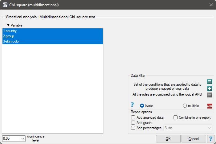
Note

This test can be calculated only on the basis of raw data.

2022/02/09 12:56

The Q-Cochran ANOVA

The Q-Cochran analysis of variance, based on the Q-Cochran test, is described by Cochran (1950)¹⁹⁾. This test is an extended McNemar test for $k\geq2$ dependent groups. It is used in hypothesis verification about symmetry between several measurements $X^{(1)}, X^{(2)},..., X^{(k)}$ for the $X$ feature. The analysed feature can have only 2 values - for the analysis, there are ascribed to them the numbers: 1 and 0.

Basic assumptions:

measurement on a nominal scale (dichotomous variables – it means the variables of two categories),
a dependent model.

Hypotheses:

$\begin{array}{cl} \mathcal{H}_0: & $all the "incompatible" observed frequencies are equal,$ \\ \mathcal{H}_1: & $not all the "incompatible" observed frequencies are equal,$ \end{array}$

where:

„incompatible” observed frequencies – the observed frequencies calculated when the value of the analysed feature is different in several measurements.

The test statistic is defined by: $\begin{displaymath} Q=\frac{(k-1)\left(kC-T^2\right)}{kT-R} \end{displaymath}$

where:

$T=\sum_{i=1}^n\sum_{j=1}^kx_{ij}$ ,

$R=\sum_{i=1}^n\left(\sum_{j=1}^kx_{ij}\right)^2$ ,

$C=\sum_{j=1}^k\left(\sum_{i=1}^nx_{ij}\right)^2$ ,

$x_{ij}$ – the value of $j$ -th measurement for $i$ -th object (so 0 or 1).

This statistic asymptotically (for large sample size) has the Chi-square distribution with a number of degrees of freedom calculated using the formula: $df=k-1$ .

The p-value, designated on the basis of the test statistic, is compared with the significance level $\alpha$ :

$\begin{array}{ccl} $ if $ p \le \alpha & \Longrightarrow & $ reject $ \mathcal{H}_0 $ and accept $ \mathcal{H}_1, \\ $ if $ p > \alpha & \Longrightarrow & $ there is no reason to reject $ \mathcal{H}_0. \\ \end{array}$

The POST-HOC tests

Introduction to the contrasts and the POST-HOC tests was performed in the unit, which relates to the one-way analysis of variance.

The Dunn test

For simple comparisons (frequency in particular measurements is always the same).

Hypotheses:

Example - simple comparisons (for the difference in proportion in a one chosen pair of measurements):

$\begin{array}{cl} \mathcal{H}_0: & $the chosen "incompatible" observed frequencies are equal,$ \\ \mathcal{H}_1: & $the chosen "incompatible" observed frequencies are different.$ \end{array}$

[i] The value of critical difference is calculated by using the following formula:

$\begin{displaymath} CD=Z_{\frac{\alpha}{c}}\sqrt{2\frac{kT-R}{n^2k(k-1)}}, \end{displaymath}$

where:

$\displaystyle Z_{\frac{\alpha}{c}}$ - is the critical value (statistic) of the normal distribution for a given significance level $\alpha$ corrected on the number of possible simple comparisons $c$ .

</WRAP

[ii] The test statistic is defined by:

$\begin{displaymath} Z=\frac{\sum_{j=1}^k c_jp_j}{\sqrt{2\frac{kT-R}{n^2k(k-1)}}}, \end{displaymath}$

where:

$p_j$ – the proportion $j$ -th measurement $(j=1,2,...k)$ ,

The test statistic asymptotically (for large sample size) has the normal distribution, and the p-value is corrected on the number of possible simple comparisons $c$ .

The settings window with the Cochran Q ANOVA can be opened in Statistics menu→ NonParametric tests→Cochran Q ANOVA or in ''Wizard''.

Note

This test can be calculated only on the basis of raw data.

EXAMPLE(test.pqs file)

We want to compare the difficulty of 3 test questions. To do this, we select a sample of 20 people from the analysed population. Every person from the sample answers 3 test questions. Next, we check the correctness of answers (an answer can be correct or wrong). In the table, there are following scores:

$\begin{tabular}{|c|c|c|c|} \hline No.&question 1 answer &question 2 answer &question 3 answer \\\hline 1&correct&correct&wrong\\ 2&wrong&correct&wrong\\ 3&correct&correct&correct\\ 4&wrong&correct&wrong\\ 5&wrong&correct&wrong\\ 6&wrong&correct&correct\\ 7&wrong&wrong&wrong\\ 8&wrong&correct&wrong\\ 9&correct&correct&wrong\\ 10&wrong&correct&wrong\\ 11&wrong&wrong&wrong\\ 12&wrong&wrong&correct\\ 13&wrong&correct&wrong\\ 14&wrong&wrong&correct\\ 15&correct&wrong&wrong\\ 16&wrong&wrong&wrong\\ 17&wrong&correct&wrong\\ 18&wrong&correct&wrong\\ 19&wrong&wrong&wrong\\ 20&correct&correct&wrong\\\hline \end{tabular}$

Hypotheses:

$\begin{array}{cl} \mathcal{H}_0: & $The individual questions received the same number of correct answers,$\\ & $in the analysed population,$\\ \mathcal{H}_1: & $There are different numbers of correct and wrong answers in individual test questions, $\\ & $in the analysed population.$ \end{array}$

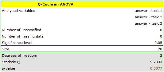
Comparing the p value p=0.0077 with the significance level $\alpha=0.05$ we conclude that individual test questions have different difficulty levels. We resume the analysis to perform POST-HOC test by clicking , and in the test option window, we select POST-HOC Dunn.

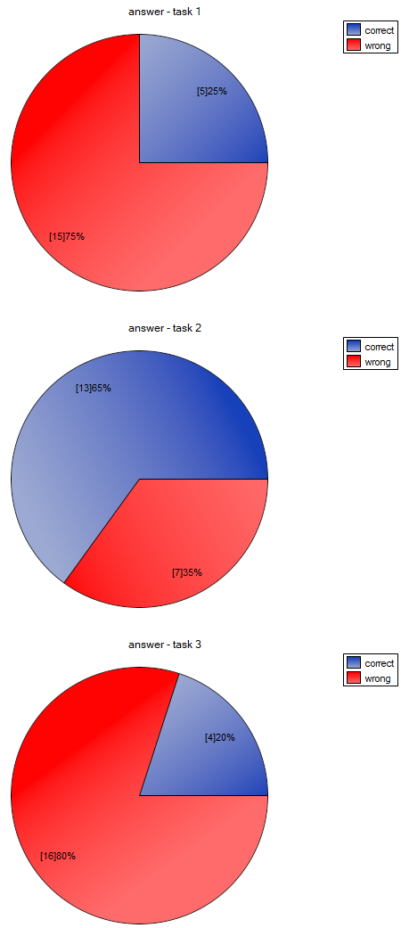
The carried out POST-HOC analysis indicates that there are differences between the 2-nd and 1-st question and between questions 2-nd and 3-th. The difference is because the second question is easier than the first and the third ones (the number of correct answers the first question is higher).

2022/02/09 12:56

¹⁾

Kruskal W.H., Wallis W.A. (1952), Use of ranks in one-criterion variance analysis. Journal of the American Statistical Association, 47, 583-621

²⁾ , ³⁾ , ¹⁰⁾

Dunn O. J. (1964), Multiple comparisons using rank sums. Technometrics, 6: 241–252

⁴⁾

Zar J. H., (2010), Biostatistical Analysis (Fifth Editon). Pearson Educational

⁵⁾ , ⁷⁾ , ¹¹⁾ , ¹³⁾

Conover W. J. (1999), Practical nonparametric statistics (3rd ed). John Wiley and Sons, New York

⁶⁾

Jonckheere A. R. (1954), A distribution-free k-sample test against ordered alternatives. Biometrika, 41: 133–145) and Terpstra (1952)((Terpstra T. J. (1952), The asymptotic normality and consistency of Kendall's test against trend, when ties are present in one ranking. Indagationes Mathematicae, 14: 327–333

⁸⁾

Friedman M. (1937), The use of ranks to avoid the assumption of normality implicit in the analysis of variance. Journal of the American Statistical Association, 32,675-701

⁹⁾

Iman R. L., Davenport J. M. (1980), Approximations of the critical region of the friedman statistic, Communications in Statistics 9, 571–595

¹²⁾

Page E. B. (1963), Ordered hypotheses for multiple treatments: A significance test for linear ranks. Journal of the American Statistical Association 58 (301): 216–30

¹⁴⁾

Durbin J. (1951), Incomplete blocks in ranking experiments. British Journal of Statistical Psychology, 4: 85–90

¹⁵⁾

Ogilvie J. C. (1965), Paired comparison models with tests for interaction. Biometrics 21(3): 651-64

¹⁶⁾ , ¹⁷⁾

Skillings J.H., Mack G.A. (1981) On the use of a Friedman-type statistic in balanced and unbalanced block designs. Technometrics, 23:171–177

¹⁸⁾

Cochran W.G. (1952), The chi-square goodness-of-fit test. Annals of Mathematical Statistics, 23, 315-345

¹⁹⁾

Cochran W.G. (1950), The comparison ofpercentages in matched samples. Biometrika, 37, 256-266

PQStat - Baza Wiedzy

Narzędzia użytkownika

Narzędzia witryny

Pasek boczny

Spis treści

Non-parametric tests

The Kruskal-Wallis ANOVA

The Jonckheere-Terpstra test for trend

The Conover ranks test of variance

The Friedman ANOVA

The Page test for trend

The Durbin's ANOVA (missing data)

The Skillings-Mack ANOVA (missing data)

The Chi-square test for multidimensional contingency tables

The Q-Cochran ANOVA

Narzędzia strony