PQStat - Baza Wiedzy

The contrasts and the POST-HOC tests

An analysis of the variance enables you to get information only if there are any significant differences among populations. It does not inform you which populations are different from each other. To gain some more detailed knowledge about the differences in particular parts of our complex structure, you should use contrasts (if you do the earlier planned and usually only particular comparisons), or the procedures of multiple comparisons POST-HOC tests (when having done the analysis of variance, we look for differences, usually between all the pairs).

The number of all the possible simple comparisons is calculated using the following formula:

$\begin{displaymath} c={k \choose 2}=\frac{k(k-1)}{2} \end{displaymath}$

Hypotheses:

The first example - simple comparisons (comparison of 2 selected means):

$\begin{array}{cc} \mathcal{H}_0: & \mu_1=\mu_2,\\ \mathcal{H}_1: & \mu_1 \neq \mu_2. \end{array}$

The second example - complex comparisons (comparison of combination of selected means):

$\begin{array}{cc} \mathcal{H}_0: & \mu_1=\frac{\mu_2+\mu_3}{2},\\[0.1cm] \mathcal{H}_1: & \mu_1\neq\frac{\mu_2+\mu_3}{2}. \end{array}$

If you want to define the selected hypothesis you should ascribe the contrast value $c_j$ , $(j=1,2,...k)$ to each mean. The $c_j$ values are selected, so that their sums of compared sides are the opposite numbers, and their values of means which are not analysed count to 0.

The first example: $c_1=1$ , $c_2=-1$ , $c_3=0, ...c_k=0$ .
The second example: $c_1=2$ , $c_2=-1$ , $c_3=-1$ , $c_4=0$ ,…, $c_k=0$ .

How to choose the proper hypothesis:

[i] Comparing the differences between the selected means with the critical difference (CD) calculated using the proper POST-HOC test:

$\begin{array}{ccl} $ if the differences between means $ \ge CD & \Longrightarrow & $ reject $ \mathcal{H}_0 $ and accept $ \mathcal{H}_1, \\ $ if the differences between means $ < CD & \Longrightarrow & $ there is no reason to reject $ \mathcal{H}_0. \\ \end{array}$

[ii] The p-value, designated on the basis of the proper POST-HOC test, is compared with the significance level $\alpha$ :

$\begin{array}{ccl} $ if $ p \le \alpha & \Longrightarrow & $ reject $ \mathcal{H}_0 $ and accept $ \mathcal{H}_1, \\ $ if $ p > \alpha & \Longrightarrow & $ there is no reason to reject $ \mathcal{H}_0. \\ \end{array}$

The LSD Fisher test

For simple and complex comparisons, equal-size groups as well as unequal-size groups, when the variances are equal.

[i] The value of critical difference is calculated by using the following formula:

$\begin{displaymath} CD=\sqrt{F_{\alpha,1,df_{WG}}}\cdot \sqrt{\left(\sum_{j=1}^k \frac{c_j^2}{n_j}\right)MS_{WG}}, \end{displaymath}$

where:

$F_{\alpha,1,df_{WG}}$ - is the critical value (statistic) of the F Snedecor distribution for a given significance level $\alpha$ and degrees of freedom, adequately: 1 and $df_{WG}$ .

[ii] The test statistic is defined by:

$\begin{displaymath} t=\frac{\sum_{j=1}^k c_j\overline{x}_j}{\sqrt{\left(\sum_{j=1}^k \frac{c_j^2}{n_j}\right)MS_{WG}}}. \end{displaymath}$

The test statistic has the t-student distribution with $df_{WG}$ degrees of freedom.

The Scheffe test

For simple comparisons, equal-size groups as well as unequal-size groups, when the variances are equal.

[i] The value of a critical difference is calculated by using the following formula:

$\begin{displaymath} CD=\sqrt{F_{\alpha,df_{BG},df_{WG}}}\cdot \sqrt{(k-1)\left(\sum_{j=1}^k \frac{c_j^2}{n_j}\right)MS_{WG}}, \end{displaymath}$

where:

$F_{\alpha,df_{BG},df_{WG}}$ - is the critical value(statistic) of the F Snedecor distribution for a given significance level $\alpha$ and $df_{BG}$ and $df_{WG}$ degrees of freedom.

[ii] The test statistic is defined by:

$\begin{displaymath} F=\frac{\left(\sum_{j=1}^k c_j\overline{x}_j\right)^2}{(k-1)\left(\sum_{j=1}^k \frac{c_j^2}{n_j}\right)MS_{WG}}. \end{displaymath}$

The test statistic has the F Snedecor distribution with $df_{BG}$ and $df_{WG}$ degrees of freedom.

The Tukey test.

For simple comparisons, equal-size groups as well as unequal-size groups, when the variances are equal.

[i] The value of a critical difference is calculated by using the following formula:

$\begin{displaymath} CD=\frac{\sqrt{2}\cdot q_{\alpha,df_{WG},k} \cdot \sqrt{\left(\sum_{j=1}^k \frac{c_j^2}{n_j}\right)MS_{WG}}}{2}, \end{displaymath}$

where:

$q_{\alpha,df_{WG},k}$ - is the critical value (statistic) of the studentized range distribution for a given significance level $\alpha$ and $df_{WG}$ and $k$ degrees of freedom.

[ii] The test statistic is defined by:

$\begin{displaymath} q=\sqrt{2}\frac{\sum_{j=1}^k c_j\overline{x}_j}{\sqrt{\left(\sum_{j=1}^k \frac{c_j^2}{n_j}\right)MS_{WG}}}. \end{displaymath}$

The test statistic has the studentized range distribution with $df_{WG}$ and $k$ degrees of freedom. Info.

The algorithm for calculating the p-value and the statistic of the studentized range distribution in PQStat is based on the Lund works (1983)¹⁾. Other applications or web pages may calculate a little bit different values than PQStat, because they may be based on less precised or more restrictive algorithms (Copenhaver and Holland (1988), Gleason (1999)).

Test for trend.

The test examining the existence of a trend can be calculated in the same situation as ANOVA for independent variables, because it is based on the same assumptions, but it captures the alternative hypothesis differently - indicating in it the existence of a trend in the mean values for successive populations. The analysis of the trend in the arrangement of means is based on contrasts Fisher LSD. By building appropriate contrasts, you can study any type of trend such as linear, quadratic, cubic, etc. Below is a table of sample contrast values for selected trends.

$\begin{tabular}{|cc||c|c|c|c|c|c|c|c|c|c|} \hline &&\multicolumn{10}{c|}{Contrast}\\\hline Number of groups&Trends&$c_1$&$c_2$&$c_3$&$c_4$&$c_5$&$c_6$&$c_7$&$c_8$&$c_9$&$c_{10}$\\\hline\hline \multirow{2}{*}{3}&line&-1&0&1&&&&&&&\\ &quadratic&1&-2&1&&&&&&&\\\hline \multirow{3}{*}{4}&line&-3&-1&1&3&&&&&&\\ &quadratic&1&-1&-1&1&&&&&&\\ &cubic&-1&3&-3&1&&&&&&\\\hline \multirow{3}{*}{5}&line&-2&-1&0&1&2&&&&&\\ &quadratic&2&-1&-2&-1&2&&&&&\\ &cubic&-1&2&0&-2&1&&&&&\\\hline \multirow{3}{*}{6}&line&-5&-3&-1&1&3&5&&&&\\ &quadratic&5&-1&-4&-4&-1&5&&&&\\ &cubic&-5&7&4&-4&-7&5&&&&\\\hline \multirow{3}{*}{7}&line&-3&-2&-1&0&1&2&3&&&\\ &quadratic&5&0&-3&-4&-3&0&5&&&\\ &cubic&-1&1&1&0&-1&-1&1&&&\\\hline \multirow{3}{*}{8}&line&-7&-5&-3&-1&1&3&5&7&&\\ &quadratic&7&1&-3&-5&-5&-3&1&7&&\\ &cubic&-7&5&7&3&-3&-7&-5&7&&\\\hline \multirow{3}{*}{9}&line&-4&-3&-2&-1&0&1&2&3&4&\\ &quadratic&28&7&-8&-17&-20&-17&-8&7&28&\\ &cubic&-14&7&13&9&0&-9&-13&-7&14&\\\hline \multirow{3}{*}{10}&line&-9&-7&-5&-3&-1&1&3&5&7&9\\ &quadratic&6&2&-1&-3&-4&-4&-3&-1&2&6\\ &cubic&-42&14&35&31&12&-12&-31&-35&-14&42\\\hline \end{tabular}$

Linear trend

A linear trend, like other trends, can be analyzed by entering the appropriate contrast values. However, if the direction of the linear trend is known, simply use the For trend option and indicate the expected order of the populations by assigning them consecutive natural numbers.

The analysis is performed on the basis of linear contrast, i.e. the groups indicated according to the natural order are assigned appropriate contrast values and the statistics are calculated Fisher LSD .

With the expected direction of the trend known, the alternative hypothesis is one-sided and the one-sided $p$ -value is interpreted. The interpretation of the two-sided $p$ -value means that the researcher does not know (does not assume) the direction of the possible trend.

The p-value, designated on the basis of the test statistic, is compared with the significance level $\alpha$ :

$\begin{array}{ccl} $ if $ p \le \alpha & \Longrightarrow & $ reject $ \mathcal{H}_0 $ and accept $ \mathcal{H}_1, \\ $ if $ p > \alpha & \Longrightarrow & $ there is no reason to reject $ \mathcal{H}_0. \\ \end{array}$

Homogeneous groups.

For each post-hoc test, homogeneous groups are constructed. Each homogeneous group represents a set of groups that are not statistically significantly different from each other. For example, suppose we divided subjects into six groups regarding smoking status: Nonsmokers (NS), Passive smokers (PS), Noninhaling smokers (NI), Light smokers (LS), Moderate smokers (MS), Heavy smokers (HS) and we examine the expiratory parameters for them. In our ANOVA we obtained statistically significant differences in exhalation parameters between the tested groups. In order to indicate which groups differ significantly and which do not, we perform post-hoc tests. As a result, in addition to the table with the results of each pair of comparisons and statistical significance in the form of $p$ :

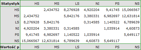
we obtain a division into homogeneous groups:

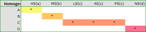
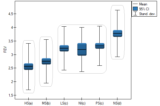
In this case we obtained 4 homogeneous groups, i.e. A, B, C and D, which indicates the possibility of conducting the study on the basis of a smaller division, i.e. instead of the six groups we studied originally, further analyses can be conducted on the basis of the four homogeneous groups determined here. The order of groups was determined on the basis of weighted averages calculated for particular homogeneous groups in such a way, that letter A was assigned to the group with the lowest weighted average, and further letters of the alphabet to groups with increasingly higher averages.

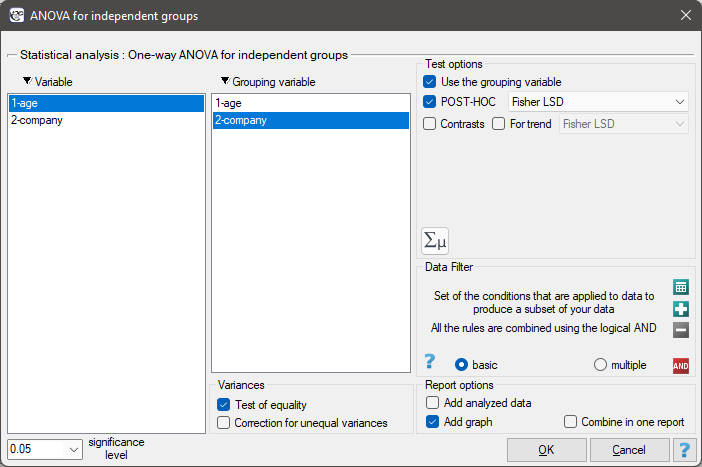
The settings window with the One-way ANOVA for independent groups can be opened in Statistics menu→Parametric tests→ANOVA for independent groups or in ''Wizard''.

¹⁾

Lund R.E., Lund J.R. (1983), Algorithm AS 190, Probabilities and Upper Quantiles for the Studentized Range. Applied Statistics; 34

PQStat - Baza Wiedzy

Narzędzia użytkownika

Narzędzia witryny

Pasek boczny

The contrasts and the POST-HOC tests

Narzędzia strony