PQStat - Baza Wiedzy

The ANOVA for dependent groups

The single-factor repeated-measures analysis of variance (ANOVA for dependent groups) is used when the measurements of an analysed variable are made several times ( $k\geq2$ ) each time in different conditions (but we need to assume that the variances of the differences between all the pairs of measurements are pretty close to each other).

This test is used to verify the hypothesis determining the equality of means of an analysed variable in several ( $k\geq2$ ) populations.

Basic assumptions:

measurement on an interval scale,
the normal distribution for all variables which are the differences of measurement pairs (or the normal distribution for an analysed variable in each measurement),
a dependent model.

Hypotheses:

$\begin{array}{cl} \mathcal{H}_0: & \mu_1=\mu_2=...=\mu_k,\\ \mathcal{H}_1: & $not all $\mu_j$ are equal $(j=1,2,...,k)$,$ \end{array}$

where:

$\mu_1$ , $\mu_2$ ,…, $\mu_k$ – means for an analysed features, in the following measurements from the examined population.

The test statistic is defined by:

$\begin{displaymath} F=\frac{MS_{BC}}{MS_{res}} \end{displaymath}$

where:

$\displaystyle MS_{BC} = \frac{SS_{BC}}{df_{BC}}$ – mean square between-conditions,

$\displaystyle MS_{res} = \frac{SS_{res}}{df_{res}}$ – mean square residual,

$\displaystyle SS_{BC} = \sum_{j=1}^k\left({\frac{\left(\sum_{i=1}^{n}x_{ij}\right)^2}{n}}\right)-\frac{\left(\sum_{j=1}^k{\sum_{i=1}^{n}x_{ij}}\right)^2}{N}$ – between-conditions sum of squares,

$\displaystyle SS_{res} = SS_{T}-SS_{BS}-SS_{BC}$ – residual sum of squares,

$\displaystyle SS_{T} = \left(\sum_{j=1}^k{\sum_{i=1}^{n}x_{ij}^2}\right)-\frac{\left(\sum_{j=1}^k{\sum_{i=1}^{n}x_{ij}}\right)^2}{N}$ – total sum of squares,

$\displaystyle SS_{BS} = \sum_{i=1}^n\left(\frac{\left(\sum_{j=1}^k x_{ij}\right)^2}{k}\right)-\frac{\left(\sum_{j=1}^k{\sum_{i=1}^{n}x_{ij}}\right)^2}{N}$ – between-subjects sum of squares,

$df_{BC}=k-1$ – between-conditions degrees of freedom,

$df_{res}=df_{T}-df_{BC}-df_{BS}$ – residual degrees of freedom,

$df_{T}=N-1$ – total degrees of freedom,

$df_{BS}=n-1$ – between-subjects degrees of freedom,

$N=nk$ ,

$n$ – sample size,

$x_{ij}$ – values of the variable from $i$ subjects $(i=1,2,...n)$ in $j$ conditions $(j=1,2,...k)$ .

The test statistic has the F Snedecor distribution with $df_{BC}$ and $df_{res}$ degrees of freedom.

The p-value, designated on the basis of the test statistic, is compared with the significance level $\alpha$ :

$\begin{array}{ccl} $ if $ p \le \alpha & \Longrightarrow & $ reject $ \mathcal{H}_0 $ and accept $ \mathcal{H}_1, \\ $ if $ p > \alpha & \Longrightarrow & $ there is no reason to reject $ \mathcal{H}_0. \\ \end{array}$

Effect size - partial <latex>$\eta^2$</latex>

This quantity indicates the proportion of explained variance to total variance associated with a factor. Thus, in a repeated measures model, it indicates what proportion of the between-conditions variability in outcomes can be attributed to repeated measurements of the variable.

$\begin{displaymath} \eta^2=\frac{SS_{BC}}{SS_{BC}+SS_{res}} \end{displaymath}$

Testy POST-HOC

Introduction to the contrasts and the POST-HOC tests was performed in the \ref{post_hoc} unit, which relates to the one-way analysis of variance.

The LSD Fisher test

For simple and complex comparisons (frequency in particular measurements is always the same).

Hypotheses:

Example - simple comparisons (comparison of 2 selected means):

$\begin{array}{cc} \mathcal{H}_0: & \mu_j=\mu_{j+1},\\ \mathcal{H}_1: & \mu_j \neq \mu_{j+1}. \end{array}$

[i] The value of the critical difference is calculated by using the following formula:

$\begin{displaymath} CD=\sqrt{F_{\alpha,1,df_{res}}}\cdot \sqrt{\left(\sum_{j=1}^k \frac{c_j^2}{n}\right)MS_{res}}, \end{displaymath}$

where:

$F_{\alpha,1,df_{res}}$ - is the critical value (statistic) of the F Snedecor distribution for a given significance level $\alpha$ and degrees of freedom, adequately: 1 and $df_{res}$ .

[ii] The test statistic is defined by:

$\begin{displaymath} t=\frac{\sum_{j=1}^k c_j\overline{x}_j}{\sqrt{\left(\sum_{j=1}^k \frac{c_j^2}{n}\right)MS_{res}}}. \end{displaymath}$

The test statistic has the t-Student distribution with $df_{res}$ degrees of freedom. Note!

For contrasts $SE_{contrast}$ is used instead of $\sqrt{\left(\sum_{j=1}^k \frac{c_j^2}{n}\right)MS_{res}}$ , and degrees of freedem: $df_{BS}$ .

The Scheffe test

For simple comparisons (frequency in particular measurements is always the same).

[i] The value of the critical difference is calculated by using the following formula:

$\begin{displaymath} CD=\sqrt{F_{\alpha,df_{BC},df_{res}}}\cdot \sqrt{(k-1)\left(\sum_{j=1}^k \frac{c_j^2}{n}\right)MS_{res}}, \end{displaymath}$

where:

$F_{\alpha,df_{BC},df_{res}}$ - is the critical value (statistic) of the F Snedecor distribution for a given significance level $\alpha$ and $df_{BC}$ and $df_{res}$ degrees of freedom.

[ $\mathfrak{(ii)}$ ] The test statistic is defined by:

$\begin{displaymath} F=\frac{\left(\sum_{j=1}^k c_j\overline{x}_j\right)^2}{(k-1)\left(\sum_{j=1}^k \frac{c_j^2}{n}\right)MS_{res}}. \end{displaymath}$ The test statistic has the F Snedecor distribution with $df_{BC}$ and $df_{ref}$ degrees of freedom.

The Tukey test.

For simple comparisons (frequency in particular measurements is always the same).

[i] The value of the critical difference is calculated by using the following formula:

$\begin{displaymath} CD=\frac{\sqrt{2}\cdot q_{\alpha,df_{res},k} \cdot \sqrt{\left(\sum_{j=1}^k \frac{c_j^2}{n}\right)MS_{res}}}{2}, \end{displaymath}$

where:

$q_{\alpha,df_{res},k}$ - is the critical value (statistic) of the studentized range distribution for a given significance level $\alpha$ and $df_{res}$ and $k$ degrees of freedom.

[ii] The test statistic is defined by:

$\begin{displaymath} q=\sqrt{2}\frac{\sum_{j=1}^k c_j\overline{x}_j}{\sqrt{\left(\sum_{j=1}^k \frac{c_j^2}{n}\right)MS_{res}}}. \end{displaymath}$

The test statistic has the studentized range distribution with $df_{res}$ and $k$ degrees of freedom.

Info.

The algorithm for calculating the p-value and statistic of the studentized range distribution in PQStat is based on the Lund works (1983)\cite{lund}. Other applications or web pages may calculate a little bit different values than PQStat, because they may be based on less precised or more restrictive algorithms (Copenhaver and Holland (1988), Gleason (1999)).

Test for trend.

The test that examines the existence of a trend can be calculated in the same situation as ANOVA for dependent variables, because it is based on the same assumptions, but it captures the alternative hypothesis differently – indicating in it the existence of a trend of mean values in successive measurements. The analysis of the trend in the arrangement of means is based on contrasts Fisher LSD test. By building appropriate contrasts, you can study any type of trend, e.g. linear, quadratic, cubic, etc. A table of example contrast values for selected trends can be found in the description of the testu dla trendu for ANOVA of independent variables.

Linear trend

Trend liniowy, tak jak pozostałe trendy, możemy analizować wpisując odpowiednie wartości kontrastów. Jeśli jednak znany jest kierunek trendu liniowego, wystarczy skorzystać z opcji Trend liniowy i wskazać oczekiwaną kolejność populacji przypisując im kolejne liczby naturalne.

A linear trend, like other trends, can be analyzed by entering the appropriate contrast values. However, if the direction of the linear trend is known, simply use the Fisher LSD test option and indicate the expected order of the populations by assigning them consecutive natural numbers.

With the expected direction of the trend known, the alternative hypothesis is one-sided and the one-sided p-values is interpreted. The interpretation of the two-sided p-value means that the researcher does not know (does not assume) the direction of the possible trend.

The p-value, designated on the basis of the test statistic, is compared with the significance level $\alpha$ :

$\begin{array}{ccl} $ if $ p \le \alpha & \Longrightarrow & $ reject $ \mathcal{H}_0 $ and accept $ \mathcal{H}_1, \\ $ if $ p > \alpha & \Longrightarrow & $ there is no reason to reject $ \mathcal{H}_0. \\ \end{array}$

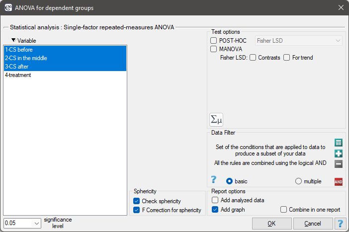
The settings window with the Single-factor repeated-measures ANOVA can be opened in Statistics menu→Parametric tests→ANOVA for dependent groups or in ''Wizard''.

EXAMPLE (pressure.pqs file)

PQStat - Baza Wiedzy

Narzędzia użytkownika

Narzędzia witryny

Pasek boczny

The ANOVA for dependent groups

Narzędzia strony