PQStat - Baza Wiedzy

The ANOVA for dependent groups with Epsilon correction and MANOVA

Epsilon and MANOVA corrections apply to repeated measurements ANOVA and are calculated when the assumption of sphericity is not met or the variances of the differences between all pairs of measurements are not close to each other.

Correction of non-sphericity

The degree to which sphericity is met is represented by the value of $W$ in the Mauchly test, but also by the values of Epsilon ( $\varepsilon$ ) calculated with corrections. $\varepsilon=1$ indicates strict adherence to the sphericity condition. The smaller the value of Epsilon is compared to 1, the more the sphericity assumption is affected. The lower limit that Epsilon can reach is $\frac{1}{k-1}$ .

To minimize the effects of non-sphericity, three corrections can be used to change the number of degrees of freedom when testing from an F distribution. The simplest but weakest is the Epsilon lower bound correction. A slightly stronger but also conservative one is the Greenhouse-Geisser correction (1959)¹⁾. The strongest is the correction by Huynh-Feldt (1976)²⁾. When sphericity is significantly affected, however, it is most appropriate to perform an analysis that does not require this assumption, namely MANOVA.

A multidimensional approach - MANOVA

MANOVA i.e. multivariate analysis of variance not assuming sphericity. If this assumption is not met, it is the most efficient method, so it should be chosen as a substitute for analysis of variance for repeated measurements. For a description of this method, see univariate MANOVA. Its use for repeated measures (without the independent groups factor) limits its application to data that are differences of adjacent measurements and provides testing of the same hypothesis as ANOVA for dependent variables. 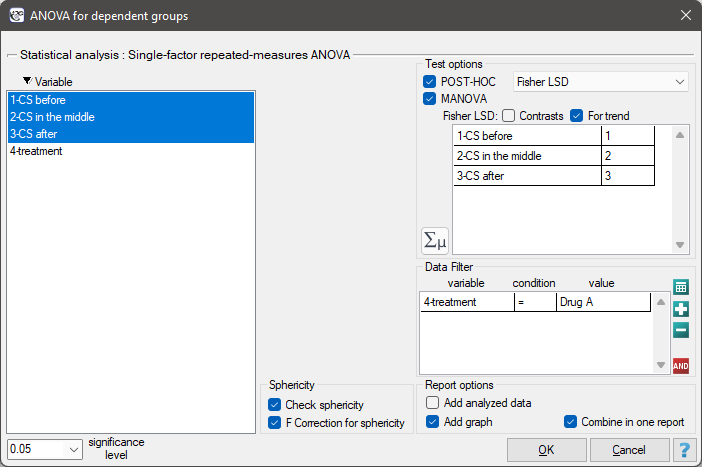Settings window for ANOVA for dependent groups with Epsilon correction and MANOVA is opened via menu Statistics→Parametric tests→ANOVA for dependent groups or via ''Wizard''.

EXAMPLE (pressure.pqs file)

The effectiveness of two treatments for hypertension was analyzed. A sample of 56 patients was collected and randomly assigned to two groups: group treated with drug A and group treated with drug B. Systolic blood pressure was measured three times in each group: before treatment, during treatment and after 6 months of treatment.

Hypotheses for treated with drug A:

$\begin{array}{cl} \mathcal{H}_0: & $Mean systolic blood pressure is the same$\\ & $at any stage of treatment - for those treated with drug A,$\\ \mathcal{H}_1: & $At least one stage of treatment with the drug A$\\ & $ mean systolic blood pressure is different.$\\ \end{array}$

The hypotheses for those treated with drug B read similar.

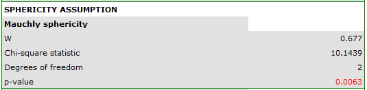
Since the data have a normal distribution, we begin our analysis by testing the assumption of sphericity. We perform the testing for each group separately using a multiple filter.

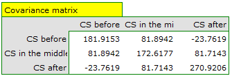
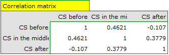
Failure to meet the sphericity assumption by the group treated with drug B is indicated by both the observed values of the covariance and correlation matrix and the result of the Mauchly test ( $W=0.68$ , p=0.0063.

We resume our analysis and in the test options window select the primary filter to perform a repeated-measures ANOVA - for those treated with drug A, followed by a correction of this analysis and a MANOVA statistic - for those treated with drug B.

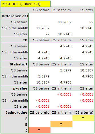
Results for those treated with drug A:

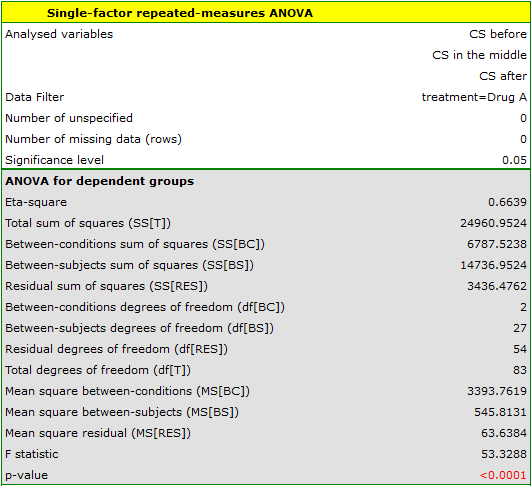
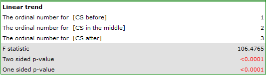
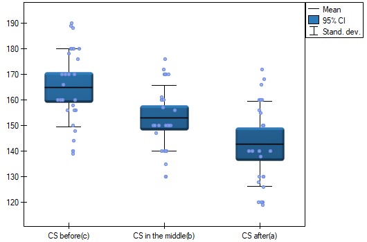
indicate significant (at the level of significance $\alpha=0.05$ ) differences between mean systolic blood pressure values (p<0.0001 for repeated measures ANOVA). More than 66% of the between-conditions variation in outcomes can be explained by the use of drug A ( $\eta=0.66$ ). The differences apply to all treatment stages compared (POST-HOC score). The decrease in systolic blood pressure due to treatment is also significant (p<0.0001). Thus, we can consider Drug A as an effective drug.

Results for those treated with drug B:

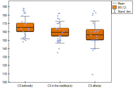
indicate that there are no significant differences between mean systolic blood pressure values, both when we use epsilon and Lambda Wilks (MANOVA) corrections. As little as 17% of the between-conditions variation in results can be explained by the use of drug B ( $\eta=0.17$ ).

¹⁾

Greenhouse S. W., Geisser S. (1959), On methods in the analysis of profile data. Psychometrika, 24, 95–112

²⁾

Huynh H., Feldt L. S. (1976), Estimation of the Box correction for degrees of freedom from sample data in randomized block and split=plot designs. Journal of Educational Statistics, 1, 69–82

PQStat - Baza Wiedzy

Narzędzia użytkownika

Narzędzia witryny

Pasek boczny

The ANOVA for dependent groups with Epsilon correction and MANOVA

Narzędzia strony