PQStat - Baza Wiedzy

Spis treści

The Mantel-Haenszel method for several tables
- The Mantel-Haenszel Odds Ratio
- The Mantel-Haenszel Relative Risk

The Mantel-Haenszel method for several tables

The Mantel-Haenszel method for $2\times2$ tables proposed by Mantel and Haenszel (1959)¹⁾ then it was extended by Mantel (1963)²⁾. A wider review the development of these methods was carried out i.a. by Newman (2001)³⁾.

This method can be used in analysis $2\times2$ tables, that occur in several ( $w>=2$ ) stratas constructed by confounding variable. For the next stratas ( $s=1,...,w$ ) the $2\times2$ contingency tables for observed frequencies are created:

$\begin{tabular}{|c|c||c|c|c|} \hline \multicolumn{2}{|c||}{Observed frequencies }& \multicolumn{3}{|c|}{Analysed phenomenon (illness)}\\\cline{3-5} \multicolumn{2}{|c||}{$s$-th strata $\left(O_{ij}^{(s)}\right)$} & occurs (case) & not occurs (control) & Total \\\hline \hline \multirow{3}{*}{Risk factor}& exposed & $O_{11}^{(s)}$ & $O_{12}^{(s)}$ & $O_{11}^{(s)}+O_{12}^{(s)}$ \\\cline{2-5} & unexposed & $O_{21}^{(s)}$ & $O_{22}^{(s)}$ & $O_{21}^{(s)}+O_{22}^{(s)}$ \\\cline{2-5} & Total & $O_{11}^{(s)}+O_{21}^{(s)}$ & $O_{12}^{(s)}+O_{22}^{(s)}$ & $n^{(s)}=O_{11}^{(s)}+O_{12}^{(s)}+O_{21}^{(s)}+O_{22}^{(s)}$\\\hline \end{tabular}$

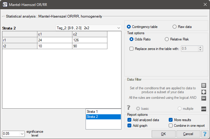
The settings window with the Mantel-Haenszel OR/RR can be opened in Statistics menu →Stratified analysis→Mantel-Haenszel OR/RR.

The Mantel-Haenszel Odds Ratio

If all tables (created by individual stratas) are homogeneous (the Chi-square test of homogeneity for the OR can check this condition), then, on the basis of these tables, the pooled odds ratio with the confidence interval can be designated. Such odds ratio, is a weighted mean for an odds ratio designated for the individual stratas. The usage of the weighted method, proposed by Mantel and Haenszel allows to include the contribution of the strata weights. Each strata has an influence on the pooled odds ratio (the greater size of the strata, the greater weight and the greater influence on the pooled odds ratio).

Weights for individual stratas are designated according to the following formula: $\begin{displaymath} g^{(s)}=\frac{O_{21}^{(s)}\cdot O_{12}^{(s)}}{n^{(s)}}, \end{displaymath}$ and the Mantel-Haenszel odds ratio: $\begin{displaymath} OR_{MH}=\frac{R}{S}, \end{displaymath}$

where:

$\displaystyle R=\sum_{s=1}^w\frac{O_{11}^{(s)}\cdot O_{22}^{(s)}}{n^{(s)}}$ ,

$\displaystyle S=\sum_{s=1}^wg^{(s)}$ .

The confidence interval for $log OR_{MH}$ is designated on the basis of the standard error (RGB – Robins-Breslow-Greenland⁴⁾⁵⁾ calculated according to the following formula:

$\begin{displaymath} SE_{MH}=\sqrt{\frac{T}{2R^2}+\frac{U+Y}{2RS}+\frac{W}{2S^2}}, \end{displaymath}$

where:

$\displaystyle T=\sum_{s=1}^wT^{(s)}$ ,\qquad $\displaystyle T^{(s)}=\frac{O_{11}^{(s)}\cdot O_{22}^{(s)}\cdot \left(O_{11}^{(s)}+O_{22}^{(s)}\right)}{\left(n^{(s)}\right)^2}$ ,

$\displaystyle U=\sum_{s=1}^wU^{(s)}$ ,\qquad $\displaystyle U^{(s)}=\frac{O_{21}^{(s)}\cdot O_{12}^{(s)}\cdot \left(O_{11}^{(s)}+O_{22}^{(s)}\right)}{\left(n^{(s)}\right)^2}$ ,

$\displaystyle Y=\sum_{s=1}^wY^{(s)}$ ,\qquad $\displaystyle Y^{(s)}=\frac{O_{11}^{(s)}\cdot O_{22}^{(s)}\cdot \left(O_{21}^{(s)}+O_{12}^{(s)}\right)}{\left(n^{(s)}\right)^2}$ ,

$\displaystyle W=\sum_{s=1}^wW^{(s)}$ ,\qquad $\displaystyle W^{(s)}=\frac{O_{21}^{(s)}\cdot O_{12}^{(s)}\cdot \left(O_{21}^{(s)}+O_{12}^{(s)}\right)}{\left(n^{(s)}\right)^2}$ .

The Mantel-Haenszel Chi-square test for the $OR_{MH}$

The Mantel-Haenszel Chi-square test for the $OR_{MH}$ is used in the hypothesis verification about the significance of designated odds ratio ( $OR_{MH}$ ). It should be calculated for large frequencies, i.e. when both conditions of the so-called „rule 5” are satisfied:

$\min(O_{11}^{(s)}+O_{12}^{(s)},O_{11}^{(s)}+O_{21}^{(s)})-\sum_{s=1}^wE_{11}^{(s)}\ge5$ for all the stratas $s=1,2,...,w$ ,
$\max(0,O_{11}^{(s)}-O_{22}^{(s)})\ge5$ for all the stratas $s=1,2,...,w$ .

When there are zero values in the table, a continuity adjustment (increasing the counts by a value of 0.5) is applied to both the observed counts and the expected counts.

Hypotheses:

$\begin{array}{cl} \mathcal{H}_0: & OR_{MH} = 1, \\ \mathcal{H}_1: & OR_{MH} \ne 1. \end{array}$

The test statistic is defined by:

$\begin{displaymath} \chi^2_{MH}=\frac{\left(\sum_{s=1}^wO_{11}^{(s)}-\sum_{s=1}^wE_{11}^{(s)}\right)^2}{V}, \end{displaymath}$

where:

$\displaystyle E_{11}^{(s)}=\frac{\left(O_{11}^{(s)}+O_{21}^{(s)}\right)\left(O_{11}^{(s)}+O_{12}^{(s)}\right)}{n^{(s)}}$ are the expected frequencies in the first contingency table cell, for the individual stratas $s=1,2,...,w$ ,

$\displaystyle V=\sum_{s=1}^wV^{(s)}$ ,

$\displaystyle V^{(s)}=\frac{\left(O_{11}^{(s)}+O_{12}^{(s)}\right)\left(O_{21}^{(s)}+O_{22}^{(s)}\right)\left(O_{11}^{(s)}+O_{21}^{(s)}\right)\left(O_{12}^{(s)}+O_{22}^{(s)}\right)}{\left(n^{(s)}\right)^2\left(n^{(s)}-1\right)}$ .

This statistic asymptotically (for large frequencies) has the Chi-square distribution with 1 degree of freedom.

The p-value, designated on the basis of the test statistic, is compared with the significance level $\alpha$ :

$\begin{array}{ccl} $ if $ p \le \alpha & \Longrightarrow & $ reject $ \mathcal{H}_0 $ and accept $ \mathcal{H}_1, \\ $ if $ p > \alpha & \Longrightarrow & $ there is no reason to reject $ \mathcal{H}_0. \\ \end{array}$

The Chi-square test of homogeneity for the $OR$

The Chi-square test of homogeneity for the $OR$ is used in the hypothesis verification that the variable, creating stratas, is the modifying effect, i.e. it influences on the designated odds ratio in the manner that, the odds ratios are significant different for individual stratas.

Hypotheses:

$\begin{array}{cl} \mathcal{H}_0: & OR_{MH} = OR^{(s)}, $ for all the stratas $s=1,2,...,w$,$ \\ \mathcal{H}_1: & OR_{MH} \ne OR^{(s)}, $ for at least one strata.$ \end{array}$

The test statistic (Breslow-Day (1980)⁶⁾, Tarone (1985)arone (1985)⁷⁾⁸⁾) is defined by:

$\begin{displaymath} \chi^2=\sum_{s=1}^w\frac{\left(O_{11}^{(s)}-E^{(s)}\right)^2}{Var^{(s)}}-\frac{\left(\sum_{s=1}^wO_{11}^{(s)}-\sum_{s=1}^wE^{(s)}\right)^2}{\sum_{s=1}^wVar^{(s)}} \end{displaymath}$

where:

$E^{(s)}$ is solution to the quadratic equation:

$\displaystyle\frac{E^{(s)}\left(O_{22}^{(s)}-O_{11}^{(s)}+E^{(s)}\right)}{\left(O_{11}^{(s)}+O_{21}^{(s)}-E^{(s)}\right)\left(O_{11}^{(s)}+O_{12}^{(s)}-E^{(s)}\right)}=OR_{MH}$ ,

$Var^{(s)}=\left(\frac{1}{E^{(s)}}+\frac{1}{O_{22}^{(s)}-O_{11}^{(s)}+E^{(s)}}+\frac{1}{O_{11}^{(s)}+O_{21}^{(s)}-E^{(s)}}+\frac{1}{O_{11}^{(s)}+O_{12}^{(s)}-E^{(s)}}\right)^{-1}$ .

This statistic asymptotically (for large frequencies) has the Chi-square distribution with the number of degrees of freedom calculated using the formula: $df=w-1$ .

The p-value, designated on the basis of the test statistic, is compared with the significance level $\alpha$ :

$\begin{array}{ccl} $ if $ p \le \alpha & \Longrightarrow & $ reject $ \mathcal{H}_0 $ and accept $ \mathcal{H}_1, \\ $ if $ p > \alpha & \Longrightarrow & $ there is no reason to reject $ \mathcal{H}_0. \\ \end{array}$

EXAMPLE (leptospirosis.pqs file)

The following table presents hypothetical poll results, conducted among inhabitants of a city and village (the village is treated as a risk factor) in West India. The poll aim was to detect risk factors of leptospirosis⁹⁾. The occurrence of leptospirosis antibodies is a indirect evidence about infection.

$\begin{tabular}{|c|c||c|c|c|} \hline \multicolumn{2}{|c||}{Observed frequencies}& \multicolumn{2}{|c|}{leptospirosis antibodies}\\\cline{3-4} \multicolumn{2}{|c||}{$O_{ij}$} & occur & not occur\\\hline \hline \multirow{3}{*}{place of residence}& rural & 60 & 140\\\cline{2-4} & urban & 60 & 140 \\\hline \end{tabular}$

The odds of the occurrence of leptospirosis antibodies, among inhabitants of the city and the village, is the same (OR=1). Let's include gender in the analysis and check what odds will be then. The sample has to be divided into 2 stratas, because of gender (they are marked in a file as a saved selection):

$\begin{tabular}{|c|c||c|c|c|} \hline \multicolumn{2}{|c||}{Observed frequencies}& \multicolumn{2}{|c|}{leptospirosis antibodies}\\\cline{3-4} \multicolumn{2}{|c||}{for men} & occur & not occur\\\hline \hline \multirow{3}{*}{place of residence}& rural & 36 & 14\\\cline{2-4} & urban & 50 & 50 \\\hline \end{tabular}$

$\begin{tabular}{|c|c||c|c|c|} \hline \multicolumn{2}{|c||}{Observed frequencies}& \multicolumn{2}{|c|}{leptospirosis antibodies}\\\cline{3-4} \multicolumn{2}{|c||}{for women} & occur & not occur\\\hline \hline \multirow{3}{*}{place of residence}& rural & 24 & 126\\\cline{2-4} & urban & 10 & 90 \\\hline \end{tabular}$

Gender is associated with both factors (the occurrence of leptospirosis anibodies and the residence in West India). This is a significant factor. Its ignorance can lead to errors in results.

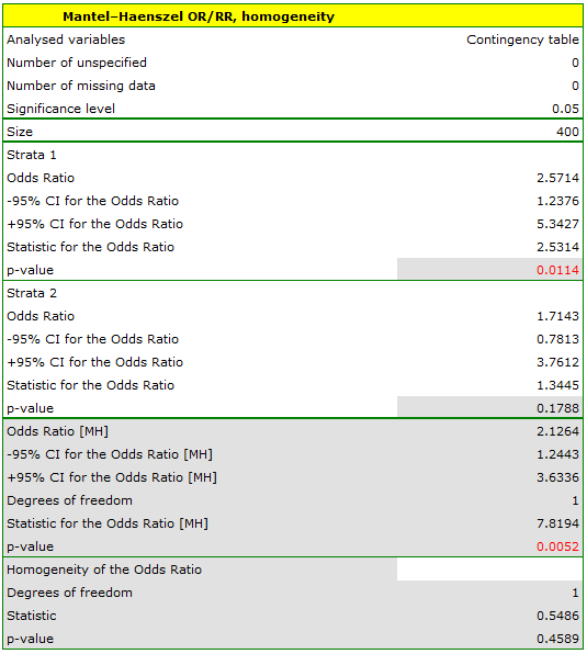
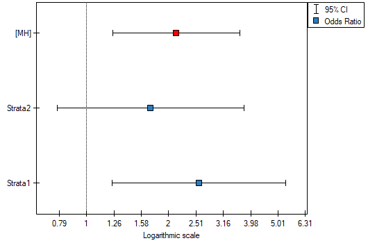
The odds of the occurrence of leptospirosis antibodies is larger among village inhabitants, both among women (OR[95%CI]=2.57[1.24, 5.34]) and men (OR[95%CI]=1.71[0.78, 3.76]). The tables are homogeneous (p=0.4589). Thus, we can use the calculated odds ratio, which is mutual for both tables ( $OR_{MH}$ [95%CI]=2.13[1.24, 3.65]). Finally, the obtained result indicates that the odds of the occurrence of leptospirosis antibodies is significantly greater among village inhabitants (p=0.0052).

2022/02/09 12:56

The Mantel-Haenszel Relative Risk

If all tables (created by individual stratas) are homogeneous (the Chi-square test of homogeneity for the RR), can check this condition), then, on the basis of these tables, the pooled relative risk with the confidence interval can be designated. Such relative risk is a weighted mean for a relative risk designated for the individual stratas. The usage of the weighted method, proposed by Mantel and Haenszel allows to include the contribution of the strata weights. Each strata of the input has an influence on the pooled relative risk construction (the greater size of the strata, the greater weight and the greater influence on the pooled relative risk).

Weights for individual stratas are designated according to the following formula:

$\begin{displaymath} g^{(s)}=\frac{O_{21}^{(s)}\left(O_{11}^{(s)}+O_{12}^{(s)}\right)}{n^{(s)}}, \end{displaymath}$

and the Mantel-Haenszel relative risk:

$\begin{displaymath} RR_{MH}=\frac{R}{S}, \end{displaymath}$

where:

$\displaystyle R=\sum_{s=1}^w\frac{O_{11}^{(s)}\left(O_{21}^{(s)}+O_{22}^{(s)}\right)}{n^{(s)}}$ ,

$\displaystyle S=\sum_{s=1}^wg^{(s)}$ .

The confidence interval for $log RR_{MH}$ is designated on the basis of the standard error calculated according to the following formula:

$\begin{displaymath} SE_{MH}=\sqrt{\frac{V}{RS}}, \end{displaymath}$

where:

$\displaystyle V=\sum_{s=1}^wV^{(s)}$ ,

$\displaystyle V^{(s)}=\frac{\left(O_{11}^{(s)}+O_{12}^{(s)}\right)\left(O_{21}^{(s)}+O_{22}^{(s)}\right)\left(O_{11}^{(s)}+O_{21}^{(s)}\right)-\left(O_{11}^{(s)}*O_{21}^{(s)}*n^{(s)}\right)}{\left(n^{(s)}\right)^2}$ .

The Manel-Hanszel Chi-square test for the $RR_{MH}$

The Mantel-Haenszel Chi-square test for the $RR_{MH}$ is used in the hypothesis verification about the significance of designated relative risk ( $RR_{MH}$ ). It should be calculated for large frequencies, in a contingency table.

Hypotheses:

$\begin{array}{cl} \mathcal{H}_0: & RR_{MH} = 1, \\ \mathcal{H}_1: & RR_{MH} \ne 1. \end{array}$

The test statistic is defined by:

$\begin{displaymath} \chi^2_{MH}=\frac{\left(\sum_{s=1}^wO_{11}^{(s)}-\sum_{s=1}^wE_{11}^{(s)}\right)^2}{V}, \end{displaymath}$

where:

$E_{11}^{(s)}=\frac{\left(O_{11}^{(s)}+O_{21}^{(s)}\right)\left(O_{11}^{(s)}+O_{12}^{(s)}\right)}{n^{(s)}}$ are the expected frequencies in the first contingency table cell, for individual stratas $s=1,2,...,w$ .

This statistic asymptotically (for large frequencies) has the Chi-square distribution with 1 degree of freedom.

The p-value, designated on the basis of the test statistic, is compared with the significance level $\alpha$ :

$\begin{array}{ccl} $ if $ p \le \alpha & \Longrightarrow & $ reject $ \mathcal{H}_0 $ and accept $ \mathcal{H}_1, \\ $ if $ p > \alpha & \Longrightarrow & $ there is no reason to reject $ \mathcal{H}_0. \\ \end{array}$

The Chi-square test of homogeneity for the $RR$

The Chi-square test of homogeneity for the $RR$ is used in the hypothesis verification that the variable creating stratas, is the modifying effect, i.e. it influences on the designated relative risk in the manner that, the relative risks are significant different for individual stratas.

Hypotheses:

$\begin{array}{cl} \mathcal{H}_0: & RR_{MH} = RR^{(s)}, $ for all the stratas $s=1,2,...,w$,$ \\ \mathcal{H}_1: & RR_{MH} \ne RR^{(s)}, $ for at least one strata.$ \end{array}$

The test statistic, using weighted least squares method, is defined by:

$\begin{displaymath} \chi^2=\sum_{s=1}^w v^{(s)}\left(\ln(RR^{(s)})-\ln(RR_{MH})\right)^2 \end{displaymath}$

where:

$v^{(s)}=\left(\frac{O_{12}^{(s)}}{O_{11}^{(s)}\left(O_{11}^{(s)}+O_{12}^{(s)}\right)}+\frac{O_{22}^{(s)}}{O_{21}^{(s)}\left(O_{21}^{(s)}+O_{22}^{(s)}\right)}\right)^{-1}$ .

This statistic asymptotically (for large frequencies) has the Chi-square distribution with the number of degrees of freedom calculated using the formula: $df=w-1$ .

The p-value, designated on the basis of the test statistic, is compared with the significance level $\alpha$ :

$\begin{array}{ccl} $ if $ p \le \alpha & \Longrightarrow & $ reject $ \mathcal{H}_0 $ and accept $ \mathcal{H}_1, \\ $ if $ p > \alpha & \Longrightarrow & $ there is no reason to reject $ \mathcal{H}_0. \\ \end{array}$

2022/02/09 12:56

¹⁾ , ²⁾

Mantel N. (1963), Chi-square tests with one degree of freedom: Extensions of the Mantel-Haenszel procedure. J. Am. Statist. Assoc., 58, 690-700

³⁾

Newman S.C.(2001), Biostatistical Methods in Epidemiology. 2nd ed. New York: John Wiley

⁴⁾

Robins, J., Breslow, N., and Greenland S. (1986), Estimators of the Mantel–Haenszel variance consistent in both sparse data and large-strata limiting models. Biometrics 42, 311–323

⁵⁾

Robins, J., Greenland S. and Breslow, N.E. (1986), A general estimator for the variance of the Mantel–Haenszel odds ratio. American Journal of Epidemiology 124, 719–723

⁶⁾

Breslow N.E., Day N.E. (1980), Statistical Methods in Cancer Research: Vol. I - The Analysis of Case-Control Studies. Lyon: International Agency for Research on Cancer

⁷⁾

Breslow N.E. (1996), Statistics in epidemiology: the case-control study', Journal of the American Statistical Association, 91, 14-28

⁸⁾

Tarone R.E. (1985), On heterogeneity tests based on efficient scores. Biometrika 72, 91–95

⁹⁾

Betty R. Kirkwood and Jonathan A. C. Sterne (2003), Medical Statistics (2nd ed.). Meassachusetts: Blackwell Science, 177-188, 240-248

PQStat - Baza Wiedzy

Narzędzia użytkownika

Narzędzia witryny

Pasek boczny

Spis treści

The Mantel-Haenszel method for several tables

The Mantel-Haenszel Odds Ratio

The Mantel-Haenszel Relative Risk

Narzędzia strony