Narzędzia użytkownika
Narzędzia witryny
Pasek boczny
en:statpqpl:plotpl:lowess
Spis treści
Local linear smoothing techniques
LOWESS
LOWESS (locally weighted scatterplot smoothing) also known as LOESS (locally estimated scatterplot smoothing) is one of many „modern” modeling methods based on the least squares method. LOESS combines the simplicity of linear regression with the flexibility of nonlinear regression. Locally weighted regression (LOESS) was independently introduced in several different fields in the late 19th and early 20th centuries (Henderson, 19161); Schiaparelli, 18662)).In the statistical literature, the method was introduced independently from different perspectives in the late 1970s by Cleveland, 19793), among others. The method used in the PQstat program is based on this particular work. The basic principle is that a smooth function can be well approximated by a low-degree polynomial (the program uses a linear function i.e., a first-degree polynomial) in the neighborhood of any point x.
Procedure algorithm:
(1)
For each point in the dataset, we build a window containing adjacent elements. The number of elements in the window is determined by the smoothing parameter  . The higher its value, the smoother the function will be. If this parameter is e.g. 0.2, then about 20\% of the data will be in the window and they will be used to build the polynomial (here the unicomial, i.e. the linear function).
Due to the need to maintain the symmetry of the window, i.e., the data in the window should be above and below the point for which we are building the model, the number of elements in the window should be odd. Therefore, the number of elements obtained from the parameter is rounded up to the first odd number. This produces a window containing an element  and the corresponding number
  of elements before and after that element in an ordered collection of data.

For example, if the window is to contain 7 elements, it will contain the element and the three preceding and three following elements of the sample. The window determined for the first and last sample elements is of the same size but the test element is not symmetrically placed in it i.e. in the middle.
(2)
At each point in the dataset, a low-degree polynomial (here a linear function) is fitted to a subset of the data located in the window. The fit is performed using a weighted least squares method, which gives more weight to points near the point whose response is estimated and less weight to points further away. In this way, a different polynomial function formula (here a linear function) is assigned to each point. The weights used in the weighted least squares method can be set quite flexibly, but points distant from the set must have less weight than points nearby. Here the weights proposed by Cleveland, the so-called tricube, are used

where the distance  from point was 0 -for points outside the designated window and was given as the actual distance between points, but normalized to the interval [0,1]-for points located within the window, so that the maximum distances in all windows were the same.
(3)
At each point, the value of the function  is computed based on the polynomial formula (here a linear function) assigned to it. Based on the points
  and the points
  estimated by this method, a smoothed function is drawn to fit the data.
Kernel smoothing
The estimation of the regression function by kernel smoothing is sometimes called the Nadaraya-Watson estimation (Nadaraya, 19644); Watson, 19645)). The kernel estimate is a weighted average of the observations within the smoothing window:

where  is the kernel function described in section Kernel estimation
The smoothing parameter  (bandwidth) has a decisive influence on the obtained estimator. The higher the value of the smoothing parameter, the greater the degree of smoothing. It is possible to choose any smoothing parameter by setting a user value. It is also possible to select it automatically by SNR, SROT or OS method. Kernel function has much less influence on the obtained result. We can choose kernels: Gaussian, uniform function (rectangle), triangular, Epanechnikov, quartic or biweight (fourth degree). A description of the different magnitudes of the smoothing parameter and kernel function can be found in the aforementioned chapter.
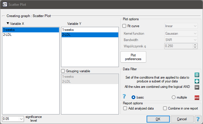
The window with the settings of the point plot options with the fitted function by the LOWESS method or by kernel smoothing can be found in various analyses. You can also make this graph via the menu Plots→Scatter Plot.
EXAMPLE continued (LDL weeks.pqs file)
The effectiveness of a new therapy designed to lower cholesterol levels in the LDL fraction was tested. 88 people at different stages of the treatment were examined. We will test whether LDL cholesterol levels decrease and stabilize as the treatment is administered over time (time in weeks).
Results are presented by initially fitting a straight line indicating the direction of the relations under study.
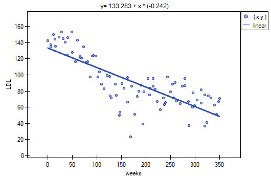
However, this way of presenting the data does not fully capture the relations taking place. From the arrangement of the points, it can be seen that the relations are initially decreasing and begins to stabilize after 150 weeks. The relations are presented again using the LOWESS method and Gaussian kernel smoothing.

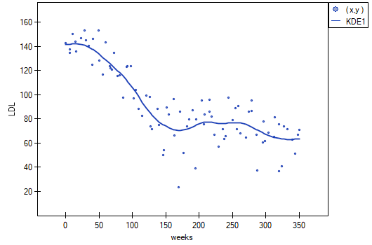
Both methods i.e., both LOWESS and kernel smoothing gave similar results and described the data much better, indicating an initial decline in LDL followed by stabilization near 70 mg/dl.
1)
Henderson, R. (1916). Note on graduation by adjusted average.Transactionsof the Actuarial Society of America, 17:43–48
2)
Schiaparelli, G. V.(1866). Sul modo di ricavare la vera espressione delle leggidelta natura dalle curve empiricae.Effemeridi Astronomiche di Milano perl’Arno, 857:3–56
3)
Cleveland, W. S. (1979). Robust Locally Weighted Regression and Smoothing Scatterplots. Journal of the American Statistical Association. 74 (368): 829–836.
4)
Nadaraya, E. A. (1964). On Estimating Regression. Theory of Probability and Its Applications. 9 (1): 141–2
5)
Watson, G. S. (1964). Smooth regression analysis. Sankhyā: The Indian Journal of Statistics, Series A. 26 (4): 359–372.
en/statpqpl/plotpl/lowess.txt · ostatnio zmienione: 2022/02/11 11:27 przez admin
Narzędzia strony
Wszystkie treści w tym wiki, którym nie przyporządkowano licencji, podlegają licencji: CC Attribution-Noncommercial-Share Alike 4.0 International
