PQStat - Baza Wiedzy

Hierarchical methods

Hierarchical cluster analysis methods involve building a hierarchy of clusters, starting from the smallest (consisting of single objects) and ending with the largest (consisting of the maximum number of objects). Clusters are created on the basis of object similarity matrix.

AGGLOMERATION PROCEDURE

By following the indicated linkage method, the algorithm finds a pair of similar objects in the similarity matrix and combines them into a cluster;
The dimension of the similarity matrix is reduced by one (two objects are replaced by one) and the distances in the matrix are recalculated;
Steps 2-3 are repeated until a single cluster containing all objects is obtained.

Object similarity

In the process of working with cluster analysis, similarity or distance measures play an essential role. The mutual similarity of objects is placed in the similarity matrix. A large variety of methods for determining the distance/similarity between objects allows to choose such measures that best reflect the actual relation. Distance and similarity measures are described in more detail in the section similarity matrix. Cluster analysis is based on finding clusters inside a similarity matrix. Such a matrix is created in the course of performing cluster analysis. For the cluster analysis to be successful, it is important to remember that higher values in the similarity matrix should indicate greater variation of objects, and lower values should indicate their similarity.

Note!

To increase the influence of the selected variables on the elements of the similarity matrix, indicate the appropriate weights when defining the distance while remembering to standardize the data.

For example, for people wanting to take care of a dog, grouping dogs according to size, coat, tail length, character, breed, etc. will make the choice easier. However, treating all characteristics identically may put completely dissimilar dogs into one group. For most of us, on the other hand, size and character are more important than tail length, so the similarity measures should be set so that size and character are most important in creating clusters.

Object and cluster linkage methods

Single linkage method - the distance between clusters is determined by the distance of those objects of each cluster that are closest to each other.

$\begin{pspicture}(-0.5,-2)(10,3) \pscircle[linewidth=2pt](.5,.5){2} \psdot[dotstyle=*](-.8,1) \psdot[dotstyle=*](1.7,0.1) \psdot[dotstyle=*](0.6,1.2) \pscircle[linewidth=2pt](6,.5){2} \psdot[dotstyle=*](7.2,1.2) \psdot[dotstyle=*](5.1,-0.4) \psdot[dotstyle=*](5.6,1.3) \psline{-}(1.7,0.1)(5.1,-0.4) \end{pspicture}$

Complete linkage method - the distance between clusters is determined by the distance of those objects of each cluster that are farthest apart.

$\begin{pspicture}(-0.5,-2)(10,3) \pscircle[linewidth=2pt](.5,.5){2} \psdot[dotstyle=*](-.8,1) \psdot[dotstyle=*](1.7,0.1) \psdot[dotstyle=*](0.6,1.2) \pscircle[linewidth=2pt](6,.5){2} \psdot[dotstyle=*](7.2,1.2) \psdot[dotstyle=*](5.1,-0.4) \psdot[dotstyle=*](5.6,1.3) \psline{-}(-.8,1)(7.2,1.2) \end{pspicture}$

Unweighted pair-group method using arithmetic averages - the distance between clusters is determined by the average distance between all pairs of objects located within two different clusters.

$\begin{pspicture}(-0.5,-2)(10,3) \pscircle[linewidth=2pt](.5,.5){2} \psdot[dotstyle=*](-.8,1) \psdot[dotstyle=*](1.7,0.1) \psdot[dotstyle=*](0.6,1.2) \pscircle[linewidth=2pt](6,.5){2} \psdot[dotstyle=*](7.2,1.2) \psdot[dotstyle=*](5.1,-0.4) \psdot[dotstyle=*](5.6,1.3) \psline{-}(-.8,1)(7.2,1.2) \psline{-}(-.8,1)(5.1,-0.4) \psline{-}(-.8,1)(5.6,1.3) \psline{-}(1.7,0.1)(7.2,1.2) \psline{-}(1.7,0.1)(5.1,-0.4) \psline{-}(1.7,0.1)(5.6,1.3) \psline{-}(0.6,1.2)(7.2,1.2) \psline{-}(0.6,1.2)(5.1,-0.4) \psline{-}(1.7,0.1)(5.6,1.3) \end{pspicture}$

Weighted pair-group metod using arithmetic averages - similarly to the unweighted pair-group method using arithmetic averages method it involves calculating the average distance, but this average is weighted by the number of elements in each cluster. As a result, we should choose this method when we expect to get clusters with similar sizes.
Ward's method - is based on the variance analysis concept - it calculates the difference between the sums of squares of deviations of distances of individual objects from the center of gravity of clusters, to which these objects belong. This method is most often chosen due to its quite universal character.

$\begin{pspicture}(-0.5,-2)(10,3) \pscircle[linewidth=2pt](.5,.5){2} \psdot[dotstyle=*](-.8,1) \psdot[dotstyle=*](1.7,0.1) \psdot[dotstyle=*](0.6,1.2) \psline[linestyle=dashed]{-}(-.8,1)(0.52,0.8) \psline[linestyle=dashed]{-}(1.7,0.1)(0.52,0.8) \psline[linestyle=dashed]{-}(0.6,1.2)(0.52,0.8) \psdot[dotstyle=pentagon*,linecolor=red](0.52,0.8) \pscircle[linewidth=2pt](6,.5){2} \psdot[dotstyle=*](7.2,1.2) \psdot[dotstyle=*](5.1,-0.4) \psdot[dotstyle=*](5.6,1.3) \psdot[dotstyle=pentagon*,linecolor=red](5.85,0.8) \psline[linestyle=dashed]{-}(7.2,1.2)(5.85,0.8) \psline[linestyle=dashed]{-}(5.1,-0.4)(5.85,0.8) \psline[linestyle=dashed]{-}(5.6,1.3)(5.85,0.8) \psline[linestyle=dotted]{-}(0.52,0.8)(5.85,0.8) \psline[linestyle=dotted]{-}(-.8,1)(7.2,1.2) \psline[linestyle=dotted]{-}(-.8,1)(5.1,-0.4) \psline[linestyle=dotted]{-}(-.8,1)(5.6,1.3) \psline[linestyle=dotted]{-}(1.7,0.1)(7.2,1.2) \psline[linestyle=dotted]{-}(1.7,0.1)(5.1,-0.4) \psline[linestyle=dotted]{-}(1.7,0.1)(5.6,1.3) \psline[linestyle=dotted]{-}(0.6,1.2)(7.2,1.2) \psline[linestyle=dotted]{-}(0.6,1.2)(5.1,-0.4) \psline[linestyle=dotted]{-}(1.7,0.1)(5.6,1.3) \end{pspicture}$

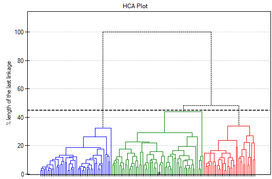
The result of a cluster analysis conducted using the hierarchical method is represented using a dendogram. A Dendogram is a form of a tree indicating the relations between particular objects obtained from the similarity matrix analysis. The cutoff level of the dendogram determines the number of clusters into which we want to divide the collected objects. The choice of the cutoff is determined by specifying the length of the bond at which the cutoff will occur as a percentage, where 100\% is the length of the last and also the longest bond in the dendogram.

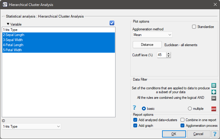
Settings window of the hierarchical cluster analysis is opened via menu Advanced Statistics→Reduction and grouping→Hierarchical Cluster Analysis.

EXAMPLE cont. (iris.pqs file)

The analysis will be performed on the classic data set of dividing iris flowers into 3 varieties based on the width and length of the petals and sepal sepals (R.A. Fisher 1936¹⁾). Because this data set contains information about the actual variety of each flower, after performing a cluster analysis it is possible to determine the accuracy of the division made.

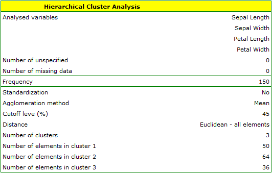
We assign flowers to particular groups on the basis of columns from 2 to 5. We choose the way of calculating distances e.g. Euclidean distance and the linkage method. Specifying the cutoff level of clusters will allow us to cut off the dendogram in such a way that clusters will be formed - in the case of this analysis we want to get 3 clusters and to achieve this we change the cutoff level to 45. We will also attach data+clusters to the report..

In the dendogram, the order of the bonds and their lengths are shown.

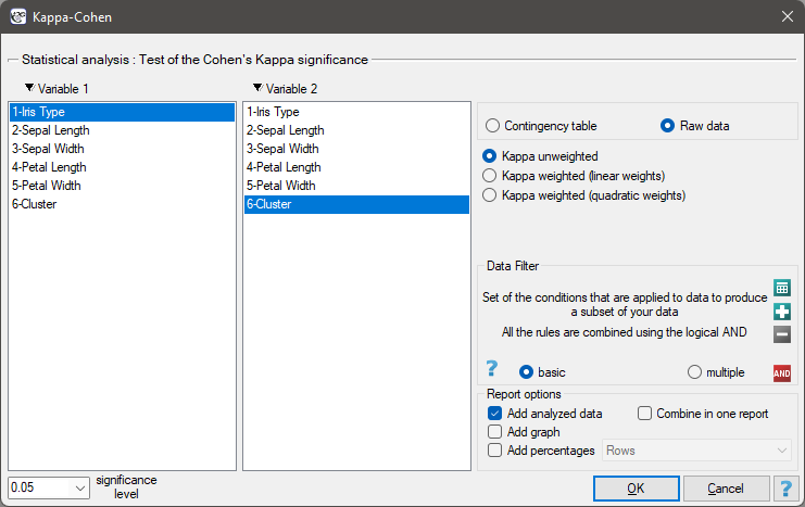
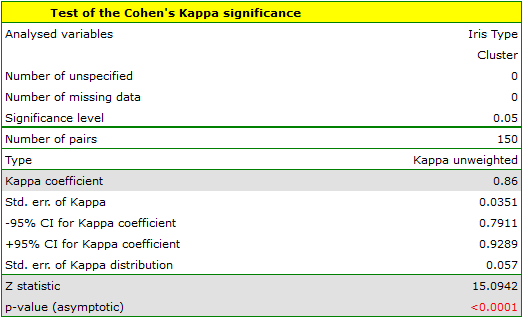
To examine whether the extracted clusters represent the 3 actual varieties of iris flowers, we can copy the column containing the information about cluster belonging from the report and paste it into the datasheet. Like the clusters, the varieties are also described numerically by Codes/Labels/Format, so we can easily perform a concordance analysis. We will check the concordance of our results with the actual belonging of a given flower to the corresponding species using the Cohen's Kappa method .

For this example, the observed concordance is shown in the table:

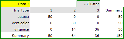
We conclude from it that the virginica variety can be confused with the versicolor variety, hence we observe 14 misclassifications. However, the Kappa concordance coefficient is statistically significant at 0.86, indicating that the clusters obtained are highly consistent with the actual flower variety.

¹⁾

Fisher R.A. (1936), The use of multiple measurements in taxonomic problems. Annals of Eugenics 7 (2): 179–188

PQStat - Baza Wiedzy

Narzędzia użytkownika

Narzędzia witryny

Pasek boczny

Hierarchical methods

Narzędzia strony