PQStat - Baza Wiedzy

The advisability of using the Principal Component Analysis

If the variables are not correlated (the Pearson's correlation coefficient is near 0), then there is no use to conduct a principal component analysis, as in such a situation every variable is already a separate component.

Bartlett's test

The test is used to verify the hypothesis that the correlation coefficients between variables are zero (i.e. the correlation matrix is an identity matrix).

Hypotheses:

$\begin{array}{cl} \mathcal{H}_0: & M = I, \\ \mathcal{H}_1: & M \ne I. \end{array}$

where:

$M$ – the variance matrix or covariance matrix of original variables $X_1,X_2,...,X_p$ ,

$I$ – the identity matrix (1 on the main axis, 0 outside of it).

The test statistic has the form presented below:

$\begin{displaymath} \chi^2=-\left(n-1-\frac{2p+5}{6}\right)\sum_{i=1}^k \ln\lambda_i, \end{displaymath}$

where:

$p$ – the number of original variables,

$n$ – size (the number of cases),

$\lambda_i$ – $i$ th eigenvalue.

That statistic has, asymptotically (for large expected frequencies), the Chi-square distribution with $p(p-1)/2$ degrees of freedom.

The p-value, designated on the basis of the test statistic, is compared with the significance level $\alpha$ :

$\begin{array}{ccl} $ if $ p \le \alpha & \Longrightarrow & $ reject $ \mathcal{H}_0 $ and accept $ \mathcal{H}_1, \\ $ if $ p > \alpha & \Longrightarrow & $ there is no reason to reject $ \mathcal{H}_0. \\ \end{array}$

The Kaiser-Meyer-Olkin coefficient

The coefficient is used to check the degree of correlation of original variables, i.e. the strength of the evidence testifying to the relevance of conducting a principal component analysis.

$\begin{displaymath} KMO=\frac{\sum_{i\ne j}^p\sum_{j\ne i}^p r_{ij}^2}{\sum_{i\ne j}^p\sum_{j\ne i}^p r_{ij}^2+\sum_{i\ne j}^p\sum_{j\ne i}^p \hat{r}_{ij}^2}, \end{displaymath}$

$r_{ij}$ – the correlation coefficient between the $i$ th and the $j$ th variable,

$\hat{r}_{ij}$ – the partial correlation coefficient between the $i$ th and the $j$ th variable.

The value of the Kaiser coefficient belongs to the range $<0,1>$ where low values testify to the lack of a need to conduct a principal component analysis, and high values are a reason for conducting such an analysis.

(file: iris.pqs)

That classical set of data was first published in Ronald Aylmer Fisher's 1936¹⁾ work in which discriminant analysis was presented. The file contains the measurements (in centimeters) of the length and width of the petals and sepals for 3 species of irises. The studied species are setosa, versicolor, and virginica. It is interesting how the species can be distinguished on the basis of the obtained measurements.

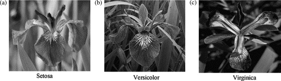
The photos are from scientific paper: Lee, et al. (2006r), „Application of a noisy data classification technique to determine the occurrence of flashover in compartment fires”

Principal component analysis will allow us to point to those measurements (the length and the width of the petals and sepals) which give the researcher the most information about the observed flowers.

The first stage of work, done even before defining and analyzing principal components, is checking the advisability of conducting the analysis. We start, then, from defining a correlation matrix of the variables and analyzing the obtained correlations with the use of Bartlett's test and the KMO coefficient.

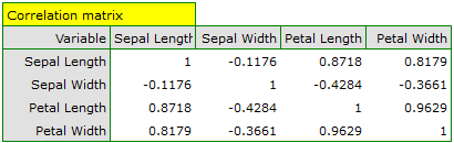
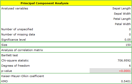
The p-value of Bartlett's statistics points to the truth of the hypothesis that there is a significant difference between the obtained correlation matrix and the identity matrix, i.e. that the data are strongly correlated. The obtained KMO coefficient is average and equals 0.54. We consider the indications for conducting a principal component analysis to be sufficient.

The first result of that analysis which merits our special attention are eigenvalues:

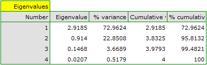
The obtained eigenvalues show that one or even two principal components will describe our data well. The eigenvalue of the first component is 2.92 and the percent of the explained variance is 72.96. The second component explains much less variance, i.e. 22.85%, and its eigenvalue is 9.91. According to Kaiser criterion, one principal component is enough for an interpretation, as only for the first principal component the eigenvalue is greater than 1. However, looking at the graph of the scree we can conclude that the decreasing line changes into a horizontal one only at the third principal component.

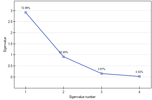
From that we may infer that the first two principal components carry important information. Together they explain a great part, as much as 95.81%, of the variance (see the cumulative % column).

The communalities for the first principal component are high for all original variables except the variable of the width of the sepal, for which they equal 21.17%. That means that if we only interpret the first principal component, only a small part of the variable of the width of the sepal would be reflected.

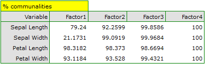
For the first two principal components the communalities are at a similar, very high level and they exceed 90% for each of the analyzed variables, which means that with the use of those components the variance of each variability is represented in over 90%.

In the light of all that knowledge it has been decided to separate and interpret 2 components.

In order to take a closer look at the relationship of principal components and original variables, that is the length and the width of the petals and sepals, we interpret: eigenvectors, factor loadings, and contributions of original variables.

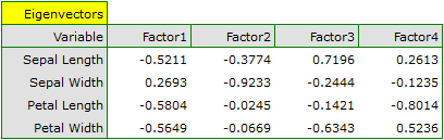
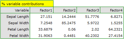
Particular original variables have differing effects on the first principal component. Let us put them in order according to that influence:

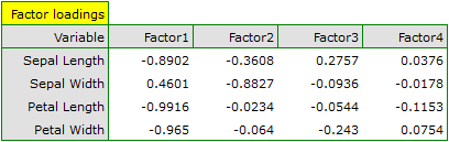
The length of a petal is negatively correlated with the first component, i.e. the longer the petal, the lower the values of that component. The eigenvector of the length of the petal is the greatest in that component and equals -0.58. Its factor loading informs that the correlation between the first principal component and the length of the petal is very high and equals -0.99 which constitutes 33.69% of the first component;
The width of the petal has an only slightly smaller influence on the first component and is also negatively correlated with it;
We interpret the length of the sepal similarly to the two previous variables but its influence on the first component is smaller;
The correlation of the width of the sepal and the first component is the weakest, and the sign of that correlation is positive.

The second component represents chiefly the original variable „sepal width”; the remaining original variables are reflected in it to a slight degree. The eigenvector, factor loading, and the contribution of the variable „sepal width” is the highest in the second component.

Each principal component defines a homogeneous group of original values. We will call the first component „petal size” as its most important variables are those which carry the information about the petal, although it has to be noted that the length of the sepal also has a significant influence on the value of that component. When interpreting we remember that the greater the values of that component, the smaller the petals.

We will call the second component „sepal width” as only the width of the sepal is reflected to a greater degree here. The greater the values of that component, the narrower the sepal.

Finally, we will generate the components by choosing, in the analysis window, the option: Add Principal Components. A part of the obtained result is presented below:

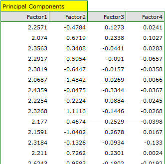
In order to be able to use the two initial components instead of the previous four original values, we copy and paste them into the data sheet. Now, the researcher can conduct the further statistics on two new, uncorrelated variables.

[Analysis of the graphs of the two initial components]

The analysis of the graphs not only leads the researcher to the same conclusions as the analysis of the tables but will also give him or her the opportunity to evaluate the results more closely.

[Factor loadings graph]

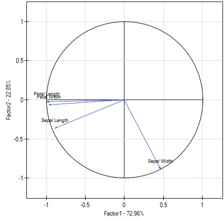
The graph shows the two first principal components which represent 72.96% of the variance and 22.85% of the variance, together amounting to 95.81% of the variance of original values

The vectors representing original values almost reach the rim of the unit circle (a circle with the radius of 1), which means they are all well represented by the two initial principal components which form the coordinate system.

The angle between the vectors illustrating the length of the petal, the width of the petal, and the length of the sepal is small, which means those variables are strongly correlated. The correlation of those variables with the components which form the system is negative, the vectors are in the third quadrant of the coordinate system. The observed values of the coordinates of the vector are higher for the first component than for the second one. Such a placement of vectors indicates that they comprise a uniform group which is represented mainly by the first component.

The vector of the width of the sepal points to an entirely different direction. It is only slightly correlated with the remaining original values, which is shown by the inclination angle with respect to the remaining original values – it is nearly a right angle. The correlation of that vector with the first component is positive and not very high (the low value of the first coordinate of the terminal point of the vector), and it is negative and high (the high value of the second coordinate of the terminal point of the vector) in the case of the second component. From that we may infer that the width of the sepal is the only original variable which is well represented by the second component.

[Biplot]

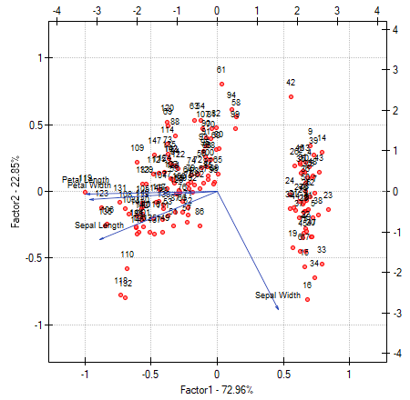
The biplot presents two series of data spread over the first two components. One series are the vectors of original values which have been presented on the previous graph and the other series are the points which carry the information about particular flowers. The values of the second series are read on the upper axis $X$ and the right axis $Y$ . The manner of interpretation of vectors, that is the first series, has been discussed with the previous graph. In order to understand the interpretation of points let us focus on flowers number 33, 34, and 109.

Flowers number 33 and 34 are similar – the distance between points 33 and 34 is small. For both points the value of the first component is much greater than the average and the value of the second component is much smaller than the average. The average value, i.e. the arithmetic mean of both components, is 0, i.e. it is the middle of the coordination system. Remembering that the first component is mainly the size of the petals and the second one is mainly the width of the sepal we can say that flowers number 33 and 34 have small petals and a large width of the sepal. Flower number 109 is represented by a point which is at a large distance from the other two points. It is a flower with a negative first component and a positive, although not high second component. That means the flower has relatively large petals while the width of the sepal is a bit smaller than average.

Similar information can be gathered by projecting the points onto the lines which extend the vectors of original values. For example, flower 33 has a large width of the sepal (high and positive values on the projection onto the original value „sepal width”) but small values of the remaining original values (negative values on the projection onto the extension of the vectors illustrating the remaining original values).

¹⁾

Fisher R.A. (1936), The use of multiple measurements in taxonomic problems. Annals of Eugenics 7 (2): 179–188

PQStat - Baza Wiedzy

Narzędzia użytkownika

Narzędzia witryny

Pasek boczny

The advisability of using the Principal Component Analysis

Narzędzia strony