PQStat - Baza Wiedzy

Spis treści

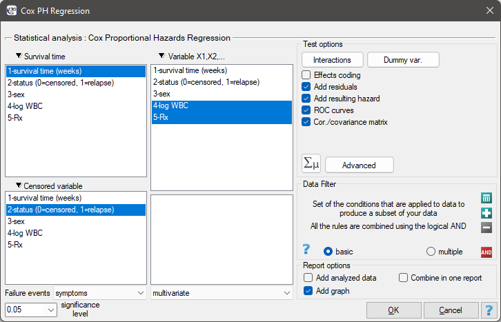
Cox proportional hazard regression

Cox proportional hazard regression

The window with settings for Cox regression is accessed via the menu Advanced statistics→Survival analysis→Cox PH regression

Cox regression, also known as the Cox proportional hazard model (Cox D.R. (1972)¹⁾), is the most popular regressive method for survival analysis. It allows the study of the impact of many independent variables ( $X_1$ , $X_2$ , $\ldots$ , $X_k$ ) on survival rates. The approach is, in a way, non-parametric, and thus encumbered with few assumptions, which is why it is so popular. The nature or shape of the hazard function does not have to be known and the only condition is the assumption which also pertains to most parametric survival models, i.e. hazard proportionality.

The function on which Cox proportional hazard model is based describes the resulting hazard and is the product of two values only one of which depends on time ( $t$ ):

$\begin{displaymath} h(t,X_1,X_2,...,X_k)=h_0(t)\cdot \exp\left(\sum_{i=1}^k\beta_iX_i\right), \end{displaymath}$

where:

$h(t,X_1,X_2,...,X_k)$ - the resulting hazard describing the risk changing in time and dependent on other factors, e.g. the treatment method,
$h_0(t)$ - the baseline hazard, i.e. the hazard with the assumption that all the explanatory variables are equal to zero,

$\sum_{i=1}^k\beta_iX_i$ - a combination (usually linear) of independent variables and model parameters,

$X_1,X_2,\ldots X_k$ - explanatory variables independent of time,

$\beta_1,\beta_2,\ldots \beta_k$ - parameters.

Dummy variables and interactions in the model

A discussion of the coding of dummy variables and interactions is presented in chapter Preparation of the variables for the analysis in multidimensional models.

Correction for ties in Cox regression is based on Breslow's method²⁾

The model can be transformed into a the linear form:

$\begin{displaymath} \ln\left(\frac{h(t,X_1,X_2,...,X_k)}{h_0(t)}\right)=\sum_{i=1}^k\beta_iX_i. \end{displaymath}$

In such a case, the solution of the equation is the vector of the estimates of parameters $\beta_0,\beta_1,\ldots,\beta_k$ called regression coefficients:

$b=\left( \begin{array}{ccc} b_1\\ b_2\\ \vdots\\ b_k \end{array}\right).$

The coefficients are estimated by the so-called partial maximum likelihood estimation. The method is called „partial” as the search for the maximum of the likelihood function $L$ (the program makes use of the Newton-Raphson iterative algorithm) only takes place for complete data; censored data are taken into account in the algorithm but not directly.

There is a certain error of estimation for each coefficient. The magnitude of that error is estimated from the following formula:

$\begin{displaymath} SE_b=\sqrt{diag(H^{-1})_b} \end{displaymath}$

where:

$diag(H^{-1})$ is the main diagonal of the covariance matrix.

Note When building a model it ought to be remembered that the number of observations should be ten times greater than or equal to the ratio of the estimated model parameters ( $k$ ) and the smaller one of the proportions of the censored or complete sizes ( $p$ ), i.e. ( $n\ge 10k/p$ ) Peduzzi P., et al(1995)³⁾.
Note When building the model you need remember that the independent variables should not be multicollinear. In a case of multicollinearity estimation can be uncertain and the obtained error values very high.
Note The criterion of convergence of the function of the Newton-Raphson iterative algorithm can be controlled with the help of two parameters: the limit of convergence iteration (it gives the maximum number of iterations in which the algorithm should reach convergence) and the convergence criterion (it gives the value below which the received improvement of estimation shall be considered to be insignificant and the algorithm will stop).

EXAMPLE cont. (remissionLeukemia.pqs file)

Hazard Ratio

An individual hazard ratio (HR) is now calculated for each independent variable : $\begin{displaymath} HR_i=e^{\beta_i}. \end{displaymath}$ It expresses the change of the risk of a failure event when the independent variable grows by 1 unit. The result is adjusted to the remaining independent variables in the model – it is assumed that they remain stable while the studied independent variable grows by 1 unit.

The $HR$ value is interpreted as follows: \item $HR >1$ means the stimulating influence of the studied independent variable on the occurrence of the failure event, i.e. it gives information about how much greater the risk of the occurrence of the failure event is when the independent variable grows by 1 unit. \item $HR <1$ means the destimulating influence of the studied independent variable on the occurrence of the failure event, i.e. it gives information about how much lower the risk is of the occurrence of the failure event when the independent variable grows by 1 unit. \item $HR\approx1$ means that the studied independent variable has no influence on the occurrence of the failure event (1). Note

If the analysis is made for a model other than linear or if interaction is taken into account, then, just as in the logistic regression model we can calculate the appropriate $HR$ on the basis of the general formula which is a combination of independent variables.

EXAMPLE cont. (remissionLeukemia.pqs file)

2022/02/09 12:56

Model verification

Statistical significance of particular variables in the model (significance of the odds ratio)

On the basis of the coefficient and its error of estimation we can infer if the independent variable for which the coefficient was estimated has a significant effect on the dependent variable. For that purpose we use Wald test.

Hypotheses:

$\begin{array}{cc} \mathcal{H}_0: & \beta_i=0,\\ \mathcal{H}_1: & \beta_i\ne 0. \end{array}$

or, equivalently:

$\begin{array}{cc} \mathcal{H}_0: & OR_i=1,\\ \mathcal{H}_1: & OR_i\ne 1. \end{array}$

The Wald test statistics is calculated according to the formula:

$\begin{displaymath} \chi^2=\left(\frac{b_i}{SE_{b_i}}\right)^2 \end{displaymath}$

The statistic asymptotically (for large sizes) has the Chi-square distribution with $1$ degree of freedom.

The p-value, designated on the basis of the test statistic, is compared with the significance level $\alpha$ :

$\begin{array}{ccl} $ if $ p \le \alpha & \Longrightarrow & $ reject $ \mathcal{H}_0 $ and accept $ \mathcal{H}_1, \\ $ if $ p > \alpha & \Longrightarrow & $ there is no reason to reject $ \mathcal{H}_0. \\ \end{array}$

The quality of the constructed model

A good model should fulfill two basic conditions: it should fit well and be possibly simple. The quality of Cox proportional hazard model can be evaluated with a few general measures based on: $L_{FM}$ - the maximum value of likelihood function of a full model (with all variables),

$L_0$ - the maximum value of the likelihood function of a model which only contains one free word,

$d$ - the observed number of failure events.

Information criteria are based on the information entropy carried by the model (model insecurity), i.e. they evaluate the lost information when a given model is used to describe the studied phenomenon. We should, then, choose the model with the minimum value of a given information criterion.

$AIC$ , $AICc$ , and $BIC$ is a kind of a compromise between the good fit and complexity. The second element of the sum in formulas for information criteria (the so-called penalty function) measures the simplicity of the model. That depends on the number of parameters ( $k$ ) in the model and the number of complete observations ( $d$ ). In both cases the element grows with the increase of the number of parameters and the growth is the faster the smaller the number of observations.

The information criterion, however, is not an absolute measure, i.e. if all the compared models do not describe reality well, there is no use looking for a warning in the information criterion.

Akaike information criterion

$\begin{displaymath} AIC=-2\ln L_{FM}+2k, \end{displaymath}$

It is an asymptomatic criterion, appropriate for large sample sizes.

Corrected Akaike information criterion

$\begin{displaymath} AICc=AIC+\frac{2k(k+1)}{d-k-1}, \end{displaymath}$

Because the correction of the Akaike information criterion concerns the sample size (the number of failure events) it is the recommended measure (also for smaller sizes).

Bayesian information criterion or Schwarz criterion

$\begin{displaymath} BIC=-2\ln L_{FM}+k\ln(d), \end{displaymath}$

Just like the corrected Akaike criterion it takes into account the sample size (the number of failure events), Volinsky and Raftery (2000)⁴⁾.

Pseudo R $^2$ - the so-called McFadden R $^2$ is a goodness of fit measure of the model (an equivalent of the coefficient of multiple determination $R^2$ defined for multiple linear regression).

The value of that coefficient falls within the range of $<0; 1)$ , where values close to 1 mean excellent goodness of fit of the model, $0$ – a complete lack of fit. Coefficient $R^2_{Pseudo}$ is calculated according to the formula:

$\begin{displaymath} R^2_{Pseudo}=1-\frac{\ln L_{FM}}{\ln L_0}. \end{displaymath}$

As coefficient $R^2_{Pseudo}$ does not assume value 1 and is sensitive to the amount of variables in the model, its corrected value is calculated:

$\begin{displaymath} R^2_{Nagelkerke}=\frac{1-e^{-(2/d)(\ln L_{FM}-\ln L_0)}}{1-e^{(2/d)\ln L_0}} \quad \textrm{or}\quad R^2_{Cox-Snell}=1-e^{\frac{(-2\ln L_0)-(-2\ln L_{FM})}{d}}. \end{displaymath}$

Statistical significance of all variables in the model

The basic tool for the evaluation of the significance of all variables in the model is the Likelihood Ratio test. The test verifies the hypothesis:

$\begin{array}{cc} \mathcal{H}_0: & \textrm{all }\beta_i=0,\\ \mathcal{H}_1: & \textrm{there is }\beta_i\neq0. \end{array}$

The test statistic has the form presented below:

$\begin{displaymath} \chi^2=-2\ln(L_0/L_{FM})=-2\ln(L_0)-(-2\ln(L_{FM})). \end{displaymath}$

The statistic asymptotically (for large sizes) has the Chi-square distribution with $k$ degrees of freedom.

The p-value, designated on the basis of the test statistic, is compared with the significance level $\alpha$ :

$\begin{array}{ccl} $ if $ p \le \alpha & \Longrightarrow & $ reject $ \mathcal{H}_0 $ and accept $ \mathcal{H}_1, \\ $ if $ p > \alpha & \Longrightarrow & $ there is no reason to reject $ \mathcal{H}_0. \\ \end{array}$

AUC - area under the ROC curve - The ROC curve – constructed based on information about the occurrence or absence of an event and the combination of independent variables and model parameters – allows us to assess the ability of the built PH Cox regression model to classify cases into two groups: (1–event) and (0–no event). The resulting curve, and in particular the area under it, illustrates the classification quality of the model. When the ROC curve coincides with the diagonal $y = x$ , the decision to assign a case to the selected class (1) or (0) made on the basis of the model is as good as randomly allocating the cases under study to these groups. The classification quality of the model is good when the curve is well above the diagonal $y=x$ , that is, when the area under the ROC curve is much larger than the area under the straight line $y=x$ , thus larger than $0.5$

Hypotheses:

$\begin{array}{cl} \mathcal{H}_0: & AUC=0.5, \\ \mathcal{H}_1: & AUC\neq 0.5. \end{array}$

The test statistic has the form:

$\begin{displaymath} Z=\frac{AUC-0.5}{SE_{0.5}}, \end{displaymath}$

where:

$SE_{0.5}$ - field error.

The statistic $Z$ has asymptotically (for large numbers) a normal distribution.

The p-value, designated on the basis of the test statistic, is compared with the significance level $\alpha$ :

$\begin{array}{ccl} $ if $ p \le \alpha & \Longrightarrow & $ reject $ \mathcal{H}_0 $ and accept $ \mathcal{H}_1, \\ $ if $ p > \alpha & \Longrightarrow & $ there is no reason to reject $ \mathcal{H}_0. \\ \end{array}$

In addition, a proposed cut-off point value for the combination of independent variables and model parameters is given for the ROC curve.

EXAMPLE cont. (remissionLeukemia.pqs file)

2022/02/09 12:56

Analysis of model residuals

The analysis of the of the model residuals allows the verification of its assumptions. The main goal of the analysis in Cox regression is the localization of outliers and the study of hazard proportionality. Typically, in regression models residuals are calculated as the differences of the observed and predicted values of the dependent variable. However, in the case of censored values such a method of determining the residuals is not appropriate. In the program we can analyze residuals described as: Martingale, deviance, and Schoenfeld. The residuals can be drawn with respect to time or independent variables.

Hazard proportionality assumption

A number of graphical methods for evaluating the goodness of fit of the proportional hazard model have been created (Lee and Wang 2003\cite{lee_wang}). The most widely used are the methods based on the model residuals. As in the case of other graphical methods of evaluating hazard proportionality this one is a subjective method. For the assumption of proportional hazard to be fulfilled, the residuals should not form any pattern with respect to time but should be randomly distributed around value 0.

Martingale – the residuals can be interpreted as a difference in time $[0,t]$ between the observed number of failure events and their number predicted by the model. The value of the expected residuals is 0 but they have a diagonal distribution which makes it more difficult to interpret the graph (they are in the range of $-\infty$ to 1).
Deviance – similarly to martingale, asymptotically they obtain value 0 but are distributed symmetrically around zero with standard deviation equal to 1 when the model is appropriate. The deviance value is positive when the studied object survives for a shorter period of time than the one expected on the basis of the model, and negative when that period is longer. The analysis of those residuals is used in the study of the proportionality of the hazard but it is mainly a tool for identifying outliers. In the residuals report those of them which are further than 3 standard deviations away from 0 are marked in red.
Schoenfeld – the residuals are calculated separately for each independent variable and only defined for complete observations. For each independent variable the sum of Shoenfeld residuals and their expected value is 0. An advantage of presenting the residuals with respect to time for each variable is the possibility of identifying a variable which does not fulfill, in the model, the assumption of hazard proportionality. That is the variable for which the graph of the residuals forms a systematic pattern (usually the studied area is the linear dependence of the residuals on time). An even distribution of points with respect to value 0 shows the lack of dependence of the residuals on time, i.e. the fulfillment of the assumption of hazard proportionality by a given variable in the model.

If the assumption of hazard proportionality is not fulfilled for any of the variables in Cox model, one possible solution is to make Cox's analyses separately for each level of that variable.

EXAMPLE cont. (remissionLeukemia.pqs file)

2022/02/09 12:56

¹⁾

Cox D.R. (1972), Regression models and life tables. Journal of the Royal Statistical Society, B34:187-220

²⁾

Breslow N.E. (1974), Covariance analysis of censored survival data. Biometrics, 30(1):89–99

³⁾

Peduzzi P., Concato J., Feinstein A.R., Holford T.R. (1995), Importance of events per independent variable in proportional hazards regression analysis. II. Accuracy and precision of regression estimates. Journal of Clinical Epidemiology, 48:1503-1510

⁴⁾

Volinsky C.T., Raftery A.E. (2000) , Bayesian information criterion for censored survival models. Biometrics, 56(1):256–262

PQStat - Baza Wiedzy

Narzędzia użytkownika

Narzędzia witryny

Pasek boczny

Spis treści

Cox proportional hazard regression

Hazard Ratio

Model verification

Analysis of model residuals

Narzędzia strony