PQStat - Baza Wiedzy

Comparison of Cox PH regression models

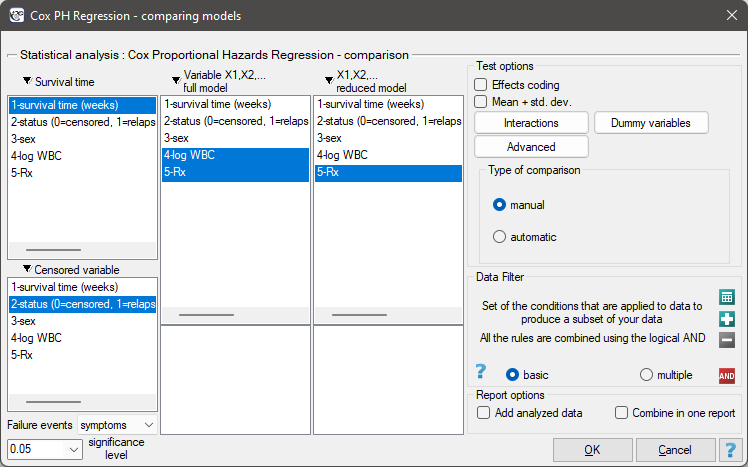
The window with settings for model comparison is accessed via the menu Advanced statistics→Survival analysis→Cox PH Regression – comparing models

Due to the possibility of simultaneous analysis of many independent variables in one Cox regression model, there is a problem of selection of an optimum model. When choosing independent variables one has to remember to put into the model variables strongly correlated with the survival time and weakly correlated with one another.

When comparing models with various numbers of independent variables we pay attention to information criteria ( $AIC$ , $AICc$ , $BIC$ ) and to goodness of fit of the model ( $R_{Pseudo}^2$ , $R^2_{Nagelkerke}$ , $R^2_{Cox-Snell}$ ). For each model we also calculate the maximum of likelihood function which we later compare with the use of the Likelihood Ratio test.

Hypotheses:

$\begin{array}{cc} \mathcal{H}_0: & L_{FM}=L_{RM},\\ \mathcal{H}_1: & L_{FM}\ne L_{RM}, \end{array}$

where:

$L_{FM}, L_{RM}$ – the maximum of likelihood function in compared models (full and reduced).

The test statistic has the form presented below:

$\begin{displaymath} \chi^2=-2\ln(L_{RM}/L_{FM})=-2\ln(L_{RM})-(-2\ln(L_{FM})) \end{displaymath}$

The statistic asymptotically (for large sizes) has the Chi-square distribution with $df=k_{FM}-k_{RM}$ degrees of freedom, where $k_{FM}$ i $k_{RM}$ is the number of estimated parameters in compared models.

The p-value, designated on the basis of the test statistic, is compared with the significance level $\alpha$ :

$\begin{array}{ccl} $ if $ p \le \alpha & \Longrightarrow & $ reject $ \mathcal{H}_0 $ and accept $ \mathcal{H}_1, \\ $ if $ p > \alpha & \Longrightarrow & $ there is no reason to reject $ \mathcal{H}_0. \\ \end{array}$

We make the decision about which model to choose on the basis of the size: $AIC$ , $AICc$ , $BIC$ , $R_{Pseudo}^2$ , $R^2_{Nagelkerke}$ , $R^2_{Cox-Snell}$ and the result of the Likelihood Ratio test which compares the subsequently created (neighboring) models. If the compared models do not differ significantly, we should select the one with a smaller number of variables. This is because a lack of a difference means that the variables present in the full model but absent in the reduced model do not carry significant information. However, if the difference is statistically significant, it means that one of them (the one with the greater number of variables) is significantly better than the other one.

In the program PQStat the comparison of models can be done manually or automatically.

Manual model comparison – construction of 2 models:

a full model – a model with a greater number of variables,
a reduced model – a model with a smaller number of variables – such a model is created from the full model by removing those variables which are superfluous from the perspective of studying a given phenomenon.

The choice of independent variables in the compared models and, subsequently, the choice of a better model on the basis of the results of the comparison, is made by the researcher.

Automatic model comparison is done in several steps:

[step 1] Constructing the model with the use of all variables.
[step 2] Removing one variable from the model. The removed variable is the one which, from the statistical point of view, contributes the least information to the current model.
[step 3] A comparison of the full and the reduced model.
[step 4] Removing another variable from the model. The removed variable is the one which, from the statistical point of view, contributes the least information to the current model.
[step 5] A comparison of the previous and the newly reduced model.
[…]

In that way numerous, ever smaller models are created. The last model only contains 1 independent variable.

EXAMPLE (remissionLeukemia.pqs file)

The analysis is based on the data about leukemia described in the work of Freirich et al. 1963¹⁾ and further analyzed by many authors, including Kleinbaum and Klein 2005²⁾. The data contain information about the time (in weeks) of remission until the moment when a patient was withdrawn from the study because of an end of remission (a return of the symptoms) or of the censorship of the information about the patient. The end of remission is the result of a failure event and is treated as a complete observation. An observation is censored if a patient remains in the study to the end and remission does not occur or if the patient leaves the study.

Patients were assigned to one of two groups: a group undergoing traditional treatment (marked as 1 and colled „placebo group”) and a group with new kind of treatment (marked as 0). The information about the patients' sex was gathered (1=man, 0=woman) and about the values of the indicator of the number of white cells, marked as „log WBC”, which is a well-known prognostic factor.

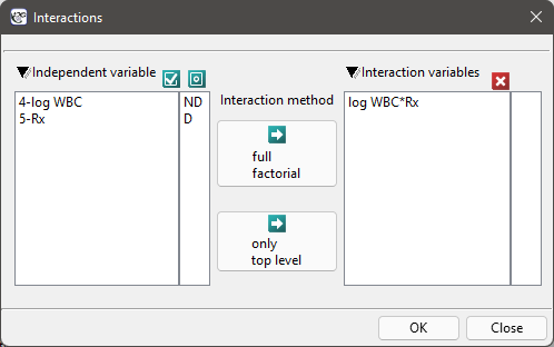
The aim of the study is to determine the influence of kind of treatment on the time of remaining in remission, taking into account possible confounding factors and interactions. In the analysis we will focus on the „Rx (1=placebo, 0=new treatment)” variable. We will place the „log WBC” variable in the model as a possible confounding factor (which modifies the effect). In order to evaluate the possible interactions of „Rx” and „log WBC” we will also consider a third variable, a ratio of the interacting variables. We will add the variable to the model by selecting, in the analysis window, the Interactions button and by setting appropriate options there.

We build three Cox models:

[Model A] only contains the „Rx” variable:

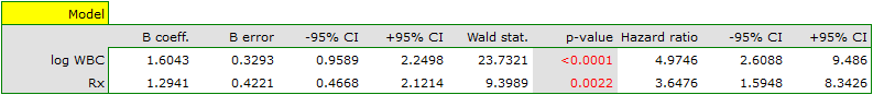
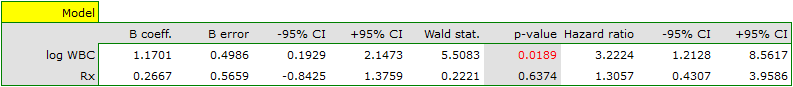
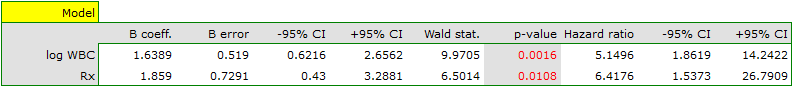
[Model B] contains the „Rx” variable and the potentially confounding variable „log WBC”:

[Model C] ontains the „Rx” variable, the „log WBC” variable, and the potential effect of the interactions of those variables: „Rx $\times$ log WBC”:

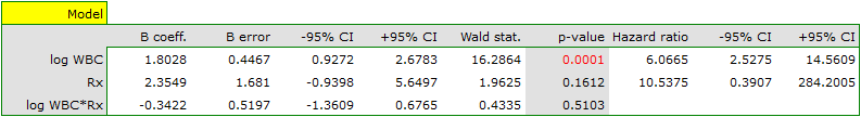
The variable which informs about the interaction of „Rx” and „log WBC”, included in model C, is not significant in model C, according to the Wald test. Thus, we can view further consideration of the interactions of the two variables in the model to be unnecessary. We will obtain similar results by comparing, with the use of a likelihood ratio test, model C with model B. We can make the comparison by choosing the Cox PH regression – comparing models menu. We will then obtain a non-significant result (p=0.5134) which means that model C (model with interaction) is NOT significantly better than model B (model without interaction).

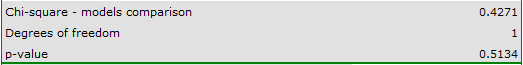
Therefore, we reject model C and move to consider model B and model A.

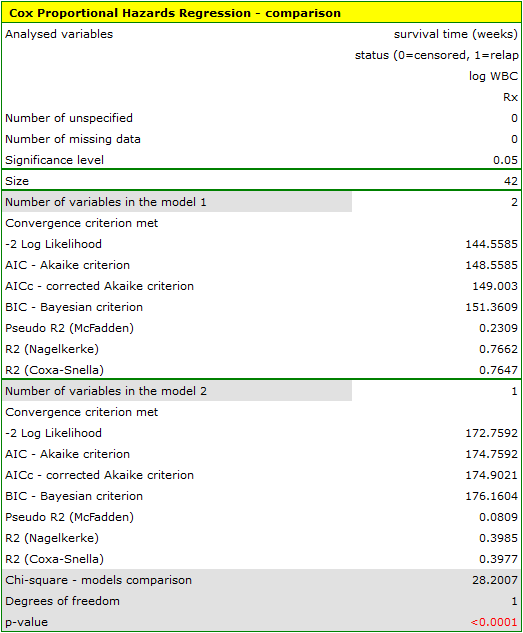
HR for „Rx” in model B is 3.65 which means that hazard for the „placebo group” is about 3.6 greater than for the patients undergoing new treatment. Model A only contains the „Rx” variable, which is why it is usually called a „crude” model – it ignores the effect of potential confounding factors. In that model the HR for „Rx” is 4.52 and is much greater than in model B. However, let us look not only at the point values of the HR estimator but also at the 95\% confidence interval for those estimators. The range for „Rx” in model A is 8.06 (10.09 minus 2.03) wide and is narrower in model B: 6.74 (8.34 minus 1.60). That is why model B gives a more precise HR estimation than model A. In order to make a final decision about which model (A or B) will be better for the evaluation of the effect of treatment („Rx”) we will once more perform a comparative analysis of the models in the Cox PH pregression – comparing models module. This time the likelihood ratio test yields a significant result (p<0.0001), which is the final confirmation of the superiority of model B. 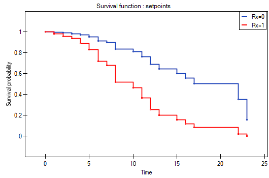That model has the lowest value of information criteria (AIC=148.6, AICc=149 BIC=151.4) and high values of goodness of fit (Pseudo $R^2_{McFadden}=0.2309$ , $R^2_{Nagelkerke}=0.7662$ , $R^2_{Cox-Snell}=0.7647$ ).

The analysis is complemented with the presentation of the survival curves of both groups, the new treatment one and the traditional treatment one, corrected by the influence of „log WBC”, for model B. In the graph we observe the differences between the groups, which occur at particular points of survival time. To plot such curves, after selecting Add Graph, we check the Survival Function: in subgroups ... and then, to quickly build a graph of two curves, I choose Quick subgroups and indicate the variable Rx. The Advanced subgroups option allows you to build any number of arbitrarily defined curves.

At the end we will evaluate the assumptions of Cox regression by analyzing the model residuals with respect to time.

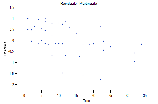
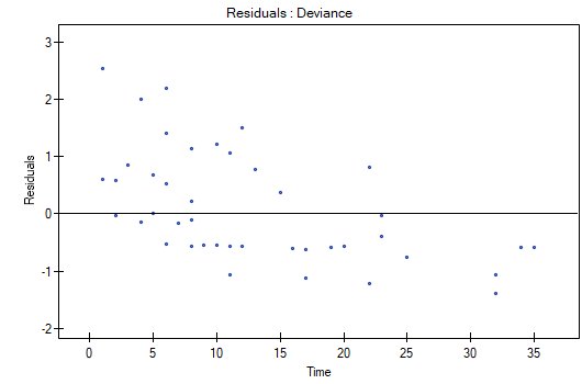
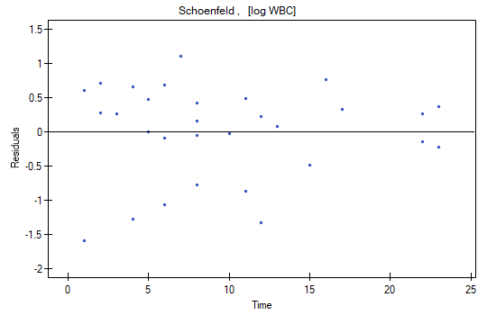
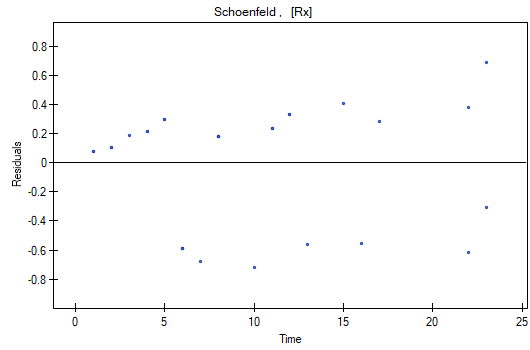
We do not observe any outliers, however, the martingale and deviance residuals become lower the longer the time. Shoenfeld residuals have a symmetrical distribution with respect to time. In their case the analysis of the graph can be supported with various tests which can evaluate if the points of the residual graph are distributed in a certain pattern, e.g. a linear dependency. In order to make such an analysis we have to copy Shoenfeld residuals, together with time, into a datasheet, and test the type of the dependence which we are looking for. The result of such a test for each variable signifies if the assumption of hazard proportionality by a variable in the model has been fulfilled. It has been fulfilled if the result is statistically insignificant and it has not been fulfilled if the result is statistically significant. As a result the variable which does not fulfill the regression assumption of the Cox proportional hazard can be excluded from the model. In the case of the „Log WBC” and „Rx” variables the symmetrical distribution of the residuals suggests the fulfillment of the assumption of hazard proportionality by those variables. That can be confirmed by checking the correlation, e.g. Pearson's linear or Spearman's monotonic, for those residuals and time.

Later we can add the sex variable to the model. However, we have to act with caution because we know, from various sources, that sex can have an influence on the survival function as regards leukemia, in that survival functions can be distributed disproportionately with respect to each other along the time line. That is why we create the Cox model for three variables: „Sex”, „Rx”, and „log WBC”. Before interpreting the coefficients of the model we will check Schonfeld residuals. We will present them in graphs and their results, together with time, will be copied from the report to a new data sheet where we will check the occurrence of Spearman's monotonic correlation. The obtained values are p=0.0259 (for the time and Shoenfeld residuals correlation for sex), p=0.6192 (for the time and Shoenfeld residuals correlation for log WBC), and p=0,1490 (for the time and Shoenfeld residuals correlation for Rx) which confirms that the assumption of hazard proportionality has not been fulfilled by the sex variable. Therefore, we will build the Cox models separately for women and men. For that purpose we will make the analysis twice, with the data filter switched on. First, the filter will point to the female sex (0), second, to the male sex (1).

For women

For men

¹⁾

Freireich E.O., Gehan E., Frei E., Schroeder L.R., Wolman I.J., et al. (1963), The effect of 6-mercaptopmine on the duration of steroid induced remission in acute leukemia. Blood, 21: 699–716

²⁾

Kleinbaum D. G., Klein M., (2005) Survival Analysis: A Self-Learning Text, Second Edition (Statistics for Biology and Health

PQStat - Baza Wiedzy

Narzędzia użytkownika

Narzędzia witryny

Pasek boczny

Comparison of Cox PH regression models

Narzędzia strony