PQStat - Baza Wiedzy

Spis treści

Meta-regression
- Model verification

Meta-regression

Meta-regression analysis is conducted in an analogous manner to the regression analysis described in the section Multiple Regression. In the case of meta-regression, the study objects are the individual studies, their results (e.g., odds ratios, relative risks, differences in means) constitute the dependent variable $Y$ i.e., the explained variable, and the additional conditions for conducting these studies constitute the independent variables ( $X_1$ , $X_2$ , $\ldots$ , $X_k$ ) i.e., the explanatory variables. As in traditional regression models, the independent variables may interact and those described by a nominal scale may be subject to special coding (for more information, see Preparation of the variables for analysis in multivariate models). The number of independent variables should be small, less than the number of papers on which the study is based on ( $n\ge k+1$ ).

We can perform meta-regression by choosing a fixed effect or a random effect.

Fixed effect is chosen when we assume that the studies represent one common true effect such that all factors that could perturb the magnitude of this effect are the same except for the factors tested as independent variables in the model ( $X_1$ , $X_2$ , $\ldots$ , $X_k$ ). This is a situation that occurs very rarely in real research because it requires fully controlled conditions, which is almost impossible in different studies, conducted in different locations and by different researchers. The use of fixed effect would be justified, for example, in a situation when all the tests are carried out at the same location, on the same population, changing only those conditions that are described by the characteristic being tested. For example, if we wanted to test the effect of changing temperature on changing the relative risk of disease described in each study, then all studies should be conducted on the same population under exactly the same conditions except for the change in temperature, which is the independent variable $X$ in the model.
Random effect is chosen when we assume that studies may represent slightly different populations, i.e., factors that could perturb the magnitude of the effect under study are not described in all papers (they can be assumed to be similar, but not necessarily exactly the same). Each paper provides the magnitudes of the factors we are interested in, which are involved in model building as independent variables ( $X_1$ , $X_2$ , $\ldots$ , $X_k$ ). The use of a random effect is common because individual studies are usually conducted at different locations under slightly different conditions, the variability of interest is only in the conditions that describe the factors given in the study, e.g., temperature, which will be the independent variable $X$ in the model.

Model verification

Statistical significance of individual variables in the model.

Based on the coefficient and its error, we can conclude whether the independent variable for which this coefficient was estimated has a significant effect on the final effect. For this purpose, we test the hypotheses:

$\begin{array}{cc} \mathcal{H}_0: & \beta_i=0,\\ \mathcal{H}_1: & \beta_i\ne 0. \end{array}$

Calculate the test statistic using the formula:

$\begin{displaymath} Z=\frac{b_i}{SE_{b_i}} \end{displaymath}$

Test statistics has the normal distribution.

The p value, designated on the basis of the test statistic, is compared with the significance level $\alpha$ :

$\begin{array}{ccl} $ if $ p \le \alpha & \Longrightarrow & $ reject $ \mathcal{H}_0 $ and accept $ \mathcal{H}_1, \\ $ if $ p > \alpha & \Longrightarrow & $ there is no reason to reject $ \mathcal{H}_0. \\ \end{array}$

Quality of the built model of a linear multivariate regression can be assessed by several measures.

Coefficient $R^2$ – is a measure of model fit. It expresses the percentage of variability between study effects explained by the model.

The value of this coefficient is in the range $<0; 1>$ , where 1 means a perfect fit of the model, 0 – a complete lack of fit. In determining it we use the following equation:

$\begin{displaymath} R^2=T^2_{(modelu)}+T^2_{(total)}, \end{displaymath}$

where:

$T^2_{(modelu)}$ – variance between studies explained by the model,

$T^2_{(total)}$ – total variance between studies.

Coefficient $I^2$ – determines the percentage of the observed variance that results from the true difference in the magnitude of the effects under study.

Note

For a detailed representation of the variance described by the coefficients, see chapter Testing heterogeneity

Statistical significance of all variables in the model

The primary tool for estimating the significance of all variables in the model is an ANOVA that determines $Q$ (of the model).

$\begin{array}{cc} \mathcal{H}_0: & \textrm{all } \beta_i=0,\\ \mathcal{H}_1: & \textrm{exists }\beta_i\neq0. \end{array}$

Using the ANOVA approach, the observed variance between tests is broken into the variance explained by the model and the variance of the residual (not explained by the model). As a result, the following $Q$ statistics are determined:

The $Q$ statistic (of the residuals) - examines the portion of the total variance that is not explained by the model,
The $Q$ statistic (of the model) - examines the portion of the total variance that is explained by the model,
The $Q$ statistic (total) - examines the variance between all studies.

Each of the above $Q$ statistics has chi-square distribution with the appropriate number of degrees of freedom.

The p value, designated on the basis of the test statistic, is compared with the significance level $\alpha$ :

$\begin{array}{ccl} $ if $ p \le \alpha & \Longrightarrow & $ reject $ \mathcal{H}_0 $ and accept $ \mathcal{H}_1, \\ $ if $ p > \alpha & \Longrightarrow & $ there is no reason to reject $ \mathcal{H}_0. \\ \end{array}$

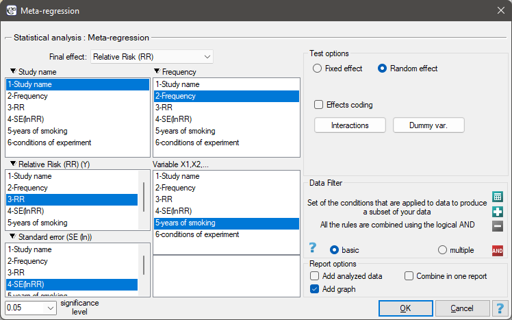
The window with settings of group comparison for meta-analysis is opened via menu: Advanced Statistics→Meta-analysis→Meta-regression.

EXAMPLE cont. (MetaAnalysisRR.pqs file)

The risk of disease X was examined for smokers and non-smokers. A meta-analysis comparing groups of studies was conducted to determine whether the number of years of smoking affected the onset of disease X and whether different conditions of the experiment resulted in different relative risks. On the basis of the comparison of the groups of studies, it was possible to establish that the last group (the group of smokers who have been smoking the longest, i.e. for more than 10 years) shows an association between smoking and the onset of disease X. On the other hand, for the groups with shorter smoking duration, no significant effect could be obtained. However, it was observed that the effect systematically increased with increasing years of smoking. To test the hypothesis of a significant increase in the risk of disease X with increasing years of smoking, two regression models were constructed. In the first model, the grouping variable Years of smoking was treated as a continuous variable. In the second model, it was determined that the variable Years of smoking would be treated as a categorical (dummy) variable with the reference group smoking less than 5 years. Data were prepared for meta-regression and stored in a file.

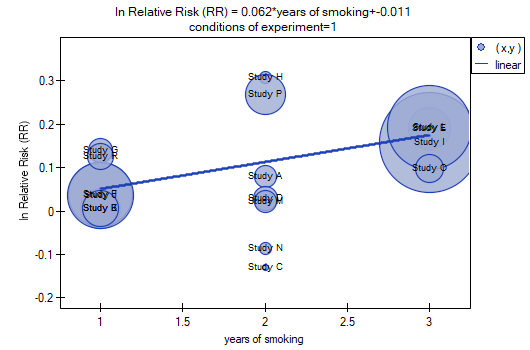
Because the papers included in the meta-analysis were from different locations and included slightly different populations, the meta-regression was performed by selecting random effect. The relative risk was selected as the final effect, and the results were presented in the graph.

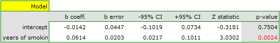
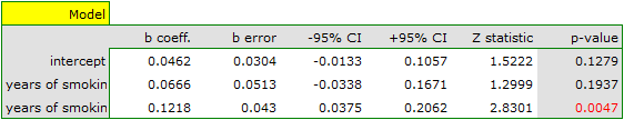
Both models confirmed a significant association between the duration of smoking and the magnitude of the relative risk of disease X. In the first model, the logarithm of the relative risk of disease X increased by 0.0614 with increasing time of smoking (moving to the subsequent group of years of smoking). Analysis of the results of the second model leads to similar conclusions. In this case, the results are considered for the group of smokers smoking less than 5 years. The logarithm of relative risk for smokers between 5 and 10 years increases by 0.0666 (relative to smokers younger than 5 years), and for smokers older than 10 years it increases by 0.1218 (relative to smokers younger than 5 years).

Since part of the study was conducted according to other criteria (under different conditions) the obtained results of both models were corrected for different conditions of the study.

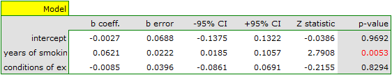
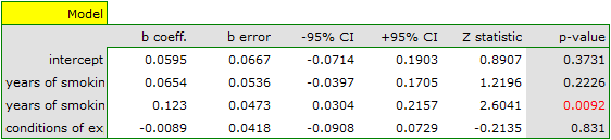
The correction performed did not change the underlying trend, and thus it can be concluded that the risk of disease X increases with years of smoking regardless of what methodology (inclusion/exclusion criteria of subjects) was used to conduct the study. The resulting relation for the first model, assuming that the study was conducted under condition „a” (indicated as first conditions) is shown in the graph.

2022/02/09 12:56

PQStat - Baza Wiedzy

Narzędzia użytkownika

Narzędzia witryny

Pasek boczny

Spis treści

Meta-regression

Model verification

Narzędzia strony